📊 SWMM 5 Complexity Index 📊

📊 SWMM 5 Complexity Index 📊

The SWMM 5 Complexity Index offers a way to measure a model's intricacy against a benchmark: the first Extran example in Extran 3, now referred to as network #1 in this broader SWMM 5 context. The foundational network showcases 22 objects and runs simulations over 8 hours. 🕗 Notably, it took 5 minutes to process this network on an IBM AT back in 1988. 🖥️⏳

The core aim of this complexity index? To provide a comparative tool for contemporary models. 📈🔄 The complexity formula evaluates the object count in the new model versus the baseline, while also accounting for any extensions in simulation time. 🔄🔍📏

📊 Complexity Index Breakdown 📊

The complexity index consolidates the count of various elements: raingages, subcatchments, junctions, outfalls, dividers, storages, conduits, pumps, orifices, weirs, outlets, control curves, and many more, right up to snowpack objects. 🌧️🌍🚰🔀🌊

For a more nuanced understanding, this index is then amplified by tallying pollutants across various elements like subcatchments, junctions, or weirs. Additionally, the multiplication of the number of land uses by the count of subcatchment objects is considered. 🧪🔄🌳🏘️

To gauge its relative complexity, this index is juxtaposed against network #1. This involves dividing the freshly computed complexity index by the foundational 22 objects and contrasting the new network's duration against the 8-hour benchmark of the base network. 🕗📏 The exemplified network flaunts a complexity rating of 5.2 and, impressively, executes in under a second on an Intel Dual Core Processor. 🖥️⚡

🔍 Understanding the Complexity Index

The complexity index is a comprehensive metric that sums up various components of a given hydrologic model. Specifically, it aggregates:

• Rain gauges, subcatchments, junctions, outfalls, dividers, storages, conduits, pumps, orifices, weirs, outlets, and several curve types (control, diversion, pump, rating, shape, storage, tidal), as well as time series, patterns, transects, hydrographs, aquifers, controls, climate objects, and snowpacks. 🌦️🌍🚰

• The index is then adjusted by taking into account the number of pollutants for multiple components like subcatchments, junctions, outfalls, and so forth. 🧪

• Additionally, it factors in the number of land uses multiplied by the count of subcatchment objects. 🌲🏙️

📏 Comparing the Complexity Index:

To gauge the relative complexity of a network:

1. The computed complexity index is divided by a baseline value of 22 objects. 📊
2. The duration of the new network is normalized against an 8-hour duration of a reference network. 🕗

For example, a showcased network had a complexity index of 5.2 and executed in under a second on an Intel Dual Core Processor. 💨🖥️

📂 Complexity Indices from Sample Models:

Using the EPA SWMM 5 QA/QC suite of files, the complexity indices for different models in the DATA.ZIP file are:

• USER4.INP: 88.5 📈
• USER1.INP: 7.4 📉
• USER2.INP: 55 📊
• USER3.INP: 20.1 📉
• USER5.INP: 18.5 📉

---

In essence, the complexity index provides a quantitative measure of a hydrologic model's intricacy, enabling modelers to benchmark and optimize performance efficiently. 👩‍💼🔧📊

SWMM 5 Pond Infiltration

You can model the pond infiltration indirectly by using either:

1. a Pump Type 4 (the classic SWMM 4 solution to this matter), in which the Pump simulates the pond depth - infiltration rate function,

2. alter the SWMM 5 Evap Factor for a pond so that you have seasonal or monthly variation in your infiltration loss simulated as an increase in Pan Evaporation or

3. You can use the newer SWMM 5 Outlet structure and use either a functional or tabular relationship to simulate the infiltration loss as a function of pond depth.

If you search the CHI Knowledge database you can also find some suggestions from Mike Gregory (and others) about modeling infiltration loss from a pond. I would recommend items 2 and 3 because "An outlet curve in SWMM 5 has the same functionality as a SWMM 4 Depth related pump ( Flow versus Depth) but it has the great advantage of being explicitly designed to have multiple functions; does not have the appearance of being an ad hoc solution (as a pump simulating infiltration would be to the casual viewer) and has many wonderful other features (added by Lewis Rossman) that you would not get with a strict pump link."

Here's the expanded version with emojis:

### SWMM 5 Pond Infiltration 🌊💧

You can model the pond infiltration indirectly by using either: 🤔

1\. a Pump Type 4 (the classic SWMM 4 solution to this matter), in which the Pump simulates the pond depth - infiltration rate function, 🆚

2\. alter the SWMM 5 Evap Factor for a pond so that you have seasonal or monthly variation in your infiltration loss simulated as an increase in Pan Evaporation 🌞 or

3\. You can use the newer SWMM 5 Outlet structure and use either a functional or tabular relationship to simulate the infiltration loss as a function of pond depth. 🔬

If you search the CHI Knowledge database 🔍 you can also find some suggestions from Mike Gregory (and others) about modeling infiltration loss from a pond. I would recommend items 2 and 3 because "An outlet curve in SWMM 5 has the same functionality as a SWMM 4 Depth related pump ( Flow versus Depth) but it has the great advantage of being explicitly designed to have multiple functions; does not have the appearance of being an ad hoc solution (as a pump simulating infiltration would be to the casual viewer) and has many wonderful other features (added by Lewis Rossman) that you would not get with a strict pump link." 👌

SWMM 5 Variable Time Step

SWMM 5 Variable Time Step

In the SWMM 5 Simulation Options/Dynamic Wave Options is the Variable Time Step Frame which contains the Adjustment Factor Percentage. The Adjustment Factor is a multiplication factor on the CFL condition.

The effiect of changing the Adjustment factor can be seen in the following graph. As the value of the adjustment factor changes from 75 to 50 to 25 the time step used in the program decreases because the time step gets further away from the CFL time step condition.

SWMM5 Normal Flow

Option "Define Supercritical Flow By" does inside the SWMM 5 engine. The options are called Slope, Froude and Bothin the GUI and in the engine of SWMM 5. A few other variable definitions you need to know to understand this explanation are: (1) Y1 for the upstream link depth, (2) Y2 for the downstream link depth, (3) Q for the flow in the link, (4)Qfull for the full Manning's equation flow or normal flow for the link based on the bed slope, (5) Froude1 and Froude2 for the Froude Number respectively of the upstream and downstream ends of the link, (6) n for Manning's roughness, (7) Yfull for the maximum depth of the link and (8) Qnormal for the Normal Flow equation flow based on the upstream area of the link (A1) and the upstream hydraulic radius (R1).

In the SWMM 5 engine these options are used after the dynamic wave equation flow is estimated using the St. Venant equation. The option that you choose is only active for those links that have a flow greater than 0, links with negative flow use the dynamic wave equation flow exclusively. It the flow is positive and the link is an open channel and full then the minimum of the dynamic wave flow or Qfull is used as the new flow in the link. If the flow is positive and the depth at the upstream end of the link or Y1 is less than Yfull then the engine will compare Qnormal to Q using the routines in Check Normal Flow.


If the link gets to the Check Normal Flow routines then it uses the following logic:

• If the Slope or Both option is used or either the upstream node or the downstream node of the link is an outfall AND Y1 is less than Y2 then the minimum of Q from the dynamic wave equation or Q from the Normal Flow equation is used as the current iteration flow in link, or


• If the Froude or Both option AND either the upstream Froude Number or the downstream Froude number is greater than 1 then the minimum of Q from the dynamic wave equation or Q from the Normal Flow equation is used as the current iteration flow in link. This condition is never used if either of the connecting nodes of the link are outfalls.

How does this work in the actual flow that SWMM 5 estimates for a link? Consider this example in which the link flow in blue is plotted with the Qnormal flow in red and the Q dynamic wave equation flow in purple:



Qnormal is







Qnormal is only calculated when the link is not full so in the plot a Qnormal of 0 means that the pipe was full. At other times the flow in the link was equal to Qnormal as the minimum of the dynamic equation flow or the Qnormal flow is used at each iteration in the solution process. The flow is normally bounded by the Qnormal flow in SWMM 5.0.013. Your choice of the options Slope, Froude andBoth really only impact the conditions under which this comparison is true. If you use Froude or Both then Supercritical flow at either end of the link will trigger this comparison will be the dynamic wave equation flow and the Froude number at each end of the link.

Smaller Storms Drop Larger Overall Rainfall In Hurricane Season

Smaller Storms Drop Larger Overall Rainfall In Hurricane Season

ScienceDaily (Dec. 11, 2007) — Researchers have found that when residents of the U.S. southeastern states look skyward for rain to alleviate a long-term drought, they should be hoping for a tropical storm over a hurricane for more reasons than one. According to a new study using NASA satellite data, smaller tropical storms do more to alleviate droughts than hurricanes do over the course of a season by bringing greater cumulative rainfall.

A new study that provides insight into what kind of storms are best at tackling drought in the southeastern United States. The study focuses on a decade of first-ever daily rainfall measurements by a NASA satellite carrying a weather radar in space. The study's authors believe the same insights can be applied by meteorologists and public officials to other regions where daily satellite rainfall data and storm tracking data are available.

In the wake of Hurricane Katrina, meteorologist Marshall Shepherd, an associate professor of geography and atmospheric sciences at the University of Georgia, Athens, and colleagues delved into the ongoing debate about whether global warming is leading to an increase in rainfall intensity. The researchers wanted to determine how much rainfall each type of cyclone, from tropical depressions to category five hurricanes, contributes to overall rainfall. They focused the study on the Southeast in the hope that results could be harnessed to improve drought relief information for the region. Their findings were published today in the American Geophysical Union's Geophysical Research Letters.

"As much of the Southeast experiences record drought, our findings indicate that weak tropical systems could significantly contribute to rainfall totals that can bring relief to the region," said Shepherd, lead author of the NASA-funded study. "These types of storms are significant rain producers. The larger hurricanes aren't frequent enough to produce most of the actual rain during the season and therefore are not the primary storm type that relieves drought in the region."

Shepherd created a new measurement method as an efficient way to get a real sense for how much rainfall each type of storm contributes in a given year around the coastal regions of the southeastern U.S. To do so, he had to distinguish an average rainfall day from an extreme rainfall day. Though data from NASA's Tropical Rainfall Measuring Mission (TRMM) satellite could offer daily rainfall amounts, the data could not be used to set apart whether rainfall was average or extreme for any given day.

Shepherd and his team modeled their metric on the "cooling degree day" that energy companies use to relate daily temperature to energy needs for air conditioning. A cooling degree day is found by subtracting 65 degrees from the average daily temperature. Values larger than zero give some indication whether a day was abnormally warm. Shepherd used daily rainfall data from TRMM to determine 28.9 as the base value of average daily rainfall at one of the world's wettest locations, Maui's Mount Wailea in Hawaii.

In the same way as the cooling degree day, the "millimeter day" metric is calculated by subtracting 28.9 millimeters from the average daily rainfall in each of four ocean basins along coastal areas scattered across the south near Houston and New Orleans, east of Miami and south of North Carolina. Values greater than zero indicate a so-called "wet millimeter day" of extreme rainfall.

Using daily rainfall data from the TRMM satellite from 1998-2006, Shepherd's team compared the amount of rain that fell in the basins on extreme rainfall days with the location of tropical storms from the National Hurricane Center's storm tracking database to determine how many extreme rainfall days were associated with a particular type of tropical storm.

The team found that the most extreme rainfall days occurred in September and October, two of the busiest months of the Atlantic hurricane season. They also found that though major hurricanes produced the heaviest rainfall on any given day, the smaller tropical storms and depressions collectively produced the most rainfall over the entire season. Over half of the rainfall during the hurricane season attributed to cyclones of any type came from weaker tropical depressions and storms, compared to 27 percent from category 3-5 hurricanes.

TRMM has transformed the way researchers like Shepherd measure rainfall by providing day-to-day information that did not exist before the satellite's 1997 launch. "Though we've had monthly rainfall data available since 1979 from other sources, it's the daily rainfall data that allows us to see that tropical storm days contributed most significantly to cumulative rainfall for the season due to how frequently that kind of storm occurs," said Shepherd.

"It's important in the future to build a longer record of daily rainfall to establish, with better confidence, whether trends are occurring," said Shepherd. "This study sets the stage for us to understand how much rainfall weak and strong tropical cyclones contribute annually and whether this contribution is trending upward in response to global warming-fueled growth in tropical cyclones."

Shepherd believes advances that will improve study of cyclones and rainfall are "just around the corner" with NASA's Global Precipitation Measurement satellite, scheduled for launch in 2013. An extension of TRMM's capabilities, it will measure precipitation at higher latitudes, the actual size of snow and rain particles, and distinguish between rain and snow.
Adapted from materials provided by NASA/Goddard Space Flight Center, via EurekAlert!, a service of AAAS.
Email or share this story:
Need to cite this story in your essay, paper, or report? Use one of the following formats:
APA

MLA
NASA/Goddard Space Flight Center (2007, December 11). Smaller Storms Drop Larger Overall Rainfall In Hurricane Season. ScienceDaily. Retrieved November 27, 2008, from http://www.sciencedaily.com­ /releases/2007/12/071210104022.htm

How to Make an InfoSWMM model from the DBF Files

Follow the following steps to create MY .MXD file.

1) Open an empty InfoSWMM project. Do not initialize it.

2) Save the project as MY .MXD within the folder where you have MY. ISDB

3) Initialize the project.

4) Click the reset Display button

That should create the project for you.  If you want an H2OMAP SWMM project, you can save the InfoSWMM model, and then Import it from H2OMAP SWMM.

Force Main Transition in SWMM 5

Force Main Transition between Partial and Full Flow

1. If the force main is full then the program will use either Hazen-Willams or Darcy-Weisbach to calculate the friction loss (term dq1),

2. If the force main is NOT full then the program will use Manning's Equation.


// --- compute terms of momentum eqn.:
// --- 1. friction slope term
if ( xsect->type == FORCE_MAIN && isFull )
dq1 = dt * forcemain_getFricSlope(j, fabs(v), rMid);
else dq1 = dt * Conduit[k].roughFactor / pow(rWtd, 1.33333) * fabs(v);

double forcemain_getFricSlope(int j, double v, double hrad)
//
// Input: j = link index
// v = flow velocity (ft/sec)
// hrad = hydraulic radius (ft)
// Output: returns a force main pipe's friction slope
// Purpose: computes the headloss per unit length used in dynamic wave
// flow routing for a pressurized force main using either the
// Hazen-Williams or Darcy-Weisbach flow equations.
// Note: the pipe's roughness factor was saved in xsect.sBot in
// conduit_validate() in LINK.C.
//
{
double re, f;
TXsect xsect = Link[j].xsect;
switch ( ForceMainEqn )
{
case H_W:
return xsect.sBot * pow(v, 0.852) / pow(hrad, 1.1667); //(5.0.012 - LR)
case D_W:
re = forcemain_getReynolds(v, hrad);
f = forcemain_getFricFactor(xsect.rBot, hrad, re);
return f * xsect.sBot * v / hrad;
}
return 0.0;
}

World Rainfall

SCS Rainfall Distributions and Design Storms

SCS Rainfall Distributions for H20MAP and InfoSWMM

The base file has a 24 hyetograph for SCS Type 1A and SCS Type 2 distrubutions. The total of the rainfall is 1 inch and to make a 25 year or 50 year storm you follow these steps:

1. Clone the rainfall time series and

2. Use the Field Calculator in DB Edit to change the total rainfall by using the operand in the Field Calculator dialog. For example, the picture shown below will make a 10 inch 24 hour rainfall in the new time series.

You will end up with two series: (1) the base 1 inch hyetograph and (2) the new design storm of 10 inches.

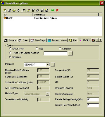
H2OMAP and InfoSWMM Sediment Transport Modeling

H2OMAP SWMM and InfoSWMM Sediment Transport Modeling

Sanitary and combined sewer systems can carry substantial loads of suspended solids (waste solids) which can accumulate and cause blockages thereby impairing the hydraulic capacity of the sewer pipes (by restricting their flow area and increasing the bed friction resistance). H2OMAP SWMM and InfoSWMM can simulate the transport and gravitational settling of (total suspended solids including grit) over time throughout the sewer collection system under varying hydraulic conditions. As long as flow velocity exceeds the critical/terminal velocity, H2OMAP SWMM and InfoSWMM assumes that the sewage flow has the capacity to transport all incoming . Deposited  particles are also assumed to be scoured and transported downstream when velocity of the sewage flow exceeds the terminal velocity. Settling starts when flow velocity falls below the critical velocity. In the model, transport of thet particles is governed by advection implying that the particles are transported at local flow velocity. 

The sediment transport modeling using H2OMAP SWMM and InfoSWMM  requires only few inputs, namely limiting flow velocity, particle settling velocity, and source node(s) and initial concentrations (in mg/l) at the source nodes. 

In order to specify the first two inputs (i.e., limiting flow velocity and particle settling velocity), the user should first select from the quality tab which in turn activates the editing tabs for particle settling velocity and limiting flow velocity. Specification of source node(s) and its/their initial concentration is similar to the method described above in relation to pollutant transport. The default values used by the model for limiting flow velocity and particle settling velocity are 2 ft/s and 0.1 ft/s, respectively.  User specified values over rid these default figures .

H2OMAP SWMM and InfoSWMM  deposition (in kg)  in pipes and  concentration (in mg/l) at manholes,  wet wells, and outlets are the outputs reported following successful simulation of  transport for a collection system.

Modified Basket Handle Cross Section Warnings

There is a rule in SWMM 5 that the depth cannot be less than half the bottom width for a modified basket handle(see below).  You always have to have a maximum depth less than 50 percent or 1/1 of the bottom width,  If you do not meet this criterion then the program will generate an invalid number warning.  This is the code from xsect.c that checks the validity of the cross section data:

    case MOD_BASKET:

        if ( p[1] <= 0.0 || p[0] <>

        xsect->yFull = p[0]/ucf;

        xsect->wMax  = p[1]/ucf;

Wave Of Sewage Flows Toward Tampa Bay

TBO > News

Wave Of Sewage Flows Toward Bay

Tribune photo by CANDACE C. MUNDY

Workers with Spectrum Underground Inc. work to repair a 20-inch sewage pipeline which broke in Town 'N Country this afternoon.

The Tampa Tribune

Published: September 13, 2008

TOWN 'N COUNTRY - Approximately 200,000 gallons of untreated sewage spilled into Sweetwater Creek on Friday afternoon, prompting a warning to residents along the creek to avoid the water, Hillsborough County officials said.

The spill occurred along Comanche Avenue just east of Hanley Road when a 20-inch sewage pipeline ruptured. The break was at a connection point to a section that had been replaced about eight weeks ago, officials said.

Because the work had been done so recently, it was under warranty, and the original contractor returned to fix the break, said Bill Bozeman, project manager for the county's water resource services. Bozeman did not know what caused it.

The fracture, reported by a passer-by at about 12:45 p.m., caused sewage to spill onto Hanley Road and ooze down Comanche toward the creek. The flow was contained two hours later. After five hours, a cloud of sewage still fogged the water along one of the creek's banks.

The section of Comanche where the spill occurred is home to a couple of businesses and a small strip of offices under construction. A narrow bridge over Sweetwater Creek leads to a neighborhood and to Sweetwater Organic Community Farm.

The farm does not rely on the creek for irrigation and the creek in that section is too shallow and choked with overgrowth in places for kayaking or swimming. County workers posted signs in English and Spanish notifying visitors of high bacterial levels and a health risk, telling them not to swim, wade or fish in the water.

Residents along the creek, which flows south to the Courtney Campbell Parkway area, are urged not to have any contact with the water for the next several days in the creek or the area where it flows into Tampa Bay.

While the contractor worked to repair the pipe, the county diverted the flow from nearby lift stations that serve the areas into tanker trucks.

The spill did not affect home use of water, Bozeman said.

The Water Resource Services staff will notify local and state environmental agencies, take samples and monitor the area where the spill occurred.

Manual de SWMM 5 en espanol

Manual de SWMM 5 en espanol

http://www.instagua.upv.es/swmm/descargas/Manual_SWMM5vE.pdf

SWMM 5 View Variables

SWMM 5 View Variables

There are four types of graphical variables in SWMM 5: (1) Subcatchements, (2) System, (3) Nodes and (4) Links.  The SWMM 5 Hydrology binary graphics file consists of 21 view variables for each subcatcment simulation in SWMM 5.  The variables are:
    

Subcatchment Variables	Description
SUBCATCH_RAINFALL	rainfall intensity
SUBCATCH_SNOWFALL	snowfall intensity
SUBCATCH_RUNOFF	total runoff flow rate
SUBCATCH_RUNOFF_IMPZero	runoff flow rate from zero imp area feb 2007
SUBCATCH_RUNOFF_IMP	runoff flow rate from imp area feb 2007
SUBCATCH_RUNOFF_Pervious	runoff flow rate from pervious area feb 2007
SUBCATCH_LOSSES	total losses (infil)
SUBCATCH_EVAP	watershed evaporation loss
SUBCATCH_DEPTH	watershed depth
SUBCATCH_GW_FLOW	groundwater flow rate to node
SUBCATCH_GW_FLOW_A1	groundwater flow rate to node
SUBCATCH_GW_FLOW_A2	groundwater flow rate to node
SUBCATCH_GW_FLOW_A3	groundwater flow rate to node
SUBCATCH_GW_ELEV	elevation of saturated gw table
SUBCATCH_GW_THETA	soil moisture
SUBCATCH_GW_PERCOLATION	aquifer deep percolation
SUBCATCH_SNOWMELT	watershed snow melt
SUBCATCH_SNOWDEPTH	watershed snow depth
SUBCATCH_FREEWATER	watershed snow depth
SUBCATCH_COLD	watershed cold content
SUBCATCH_SNOWAREA	watershed snow coverage
SUBCATCH_UL	soil thickness
SUBCATCH_FTOT	infiltration during an event
SUBCATCH_FU	current value of F
SUBCATCH_FUMAX	maximum value of F
SUBCATCH_MOISTURE	current soil mositure (less than porosity)
SUBCATCH_IMD	current IMD (Porisity - Moisture)
SUBCATCH_IMDbyEvent	IMD at the beginning of an event
SUBCATCH_SAT	Flag for saturation (1 is saturated)
SUBCATCH_INFIL_TIME	GA infiltration time
SUBCATCH_WLMAX	current infiltration RATE
SUBCATCH_NETPRECIP	rainfall intensity
SUBCATCH_BUILDUP	pollutant buildup concentration
SUBCATCH_WASHOFF	pollutant washoff concentration

The SWMM 5 system binary graphics file consists of 25 variables on one line for each system variable simulated in SWMM 5.  The variables are:

System Variables	Description
SYS_TEMPERATURE	air temperature
SYS_WINDSPEED	wind speed
SYS_RAINFALL	rainfall intensity
SYS_SNOWFALL	snow depth
SYS_RUNOFF	runoff flow
SYS_LOSSES	evap + infil
SYS_EVAP	evap
SYS_DWFLOW	dry weather inflow
SYS_GWFLOW	ground water inflow
SYS_IIFLOW	RDII inflow
SYS_EXFLOW	external inflow
SYS_INFLOW	total lateral inflow
SYS_FLOODING	flooding outflow
SYS_OUTFLOW	outfall outflow
SYS_STORAGE	storage volume
SYS_CE	continuity error for the basin
SYS_ITERATIONS	average iterations over the basin
SYS_SNOWDEPTH	snow depth
SYS_COLD	cold storage for the basin
SYS_SNOWMELT	snowmelt for the basin
SYS_RAINMELT	rainmelt for the basin
SYS_TS	time steps during the simulation
SYS_DWFLoad	total K3 line DWF load
SYS_WWFLoad	total K3 line WWF load
SYS_WWFLoadExtra	agency extra WWF Load

The SWMM 5 Node graphics binary file consists of 20 variables on one line for each junction/storage/outfall/divider  simulated in SWMM 5.  The variables are:

Node Variables	Description
NODE_DEPTH	water depth above invert
NODE_HEAD	hydraulic head
NODE_VOLUME	volume stored & ponded
NODE_LATFLOW	lateral inflow rate
NODE_IIFLOW	total rdii inflow rate
NODE_UH1	total rdii inflow rate from UH 1
NODE_UH2	total rdii inflow rate from UH 2
NODE_UH3	total rdii inflow rate from UH 3
NODE_DWFFLOW	total DWF inflow rate
NODE_INFLOW	total inflow rate
NODE_OUTFLOW	total outflow rate
NODE_OVERFLOW	overflow rate
NODE_CE	node ce
NODE_AREA	node surface area
NODE_DQDH	node surcharge dqdh
NODE_DENOM	node surcharge dqdh
NODE_ITERATIONS	node iterations to this time step
NODE_TIMESTEP	node iterations to this time step
NODE_CONVERGENCE	node iterations to this time step
NODE_QUAL	concentration of each pollutant

Link Variables

How Much Can You Learn From a Home DNA Test?

How much does your DNA determine your future? Our reporter has her DNA analyzed by three different labs, and shares every detail of the results... as well as how she copes with them.

read more | digg story

EMC Washoff in SWMM5

There are four steps to using EMC concentrations in your network:

1. Define your pollutant by adding a pollutant using the Data=>Quality=>Pollutant command:

2. Define the Land Use by using the Data=>Land Uses command or the Land Use Editor:

3. Define Buildup to be None by clicking on the None Tab:

4. Define the EMC Washoff concentration by clicking on the Washoff Tab:

This is where you would add a GW concentration

More: http://www.swmm2000.com/

Hurricane Dennis Tampa 2005