Link Area Types in SWMM 5

Note: There are 7 Link flow classification classes that are used to assign the area of the link to the upstream and downstream nodes of the link. The classes used during the simulation of the model are shown in the Link Classification Table in the RPT Report File. The supercritical class is the same as the subcritical assignment. The supercritical is a class of subcritical with a Froude number over 1.

Link Area Types in SWMM 5, InfoSWMM and H2OMap SWMM by dickinsonre

Note:  There are 7 Link flow classification classes that are used to assign the area of the link to the upstream and downstream nodes of the link.  The classes used during the simulation of the model are shown in the Link Classification Table in the RPT Report File.  The supercritical class is the same as the subcritical assignment.  The supercritical is a class of subcritical with a Froude number over 1.

Class	Description	Link Area Assignment
0      Dry conduit		1/2 Upstream and 1/2 Downstream Node
1      Upstream end is dry		1/2 Downstream Node
2      Downstream end is dry		1/2 Upstream Node
3      Sub-critical flow		1/2 Upstream and 1/2 Downstream Node
4      Super-critical flow		1/2 Upstream and 1/2 Downstream Node
5      Free-fall at upstream end		1/2 Downstream Node
6      Free-fall at downstream end		1/2 Upstream Node

via Blogger http://www.swmm5.net/2013/07/link-area-types-in-swmm-5-infoswmm-and.html

Class	Description	Link Area Assignment
0 Dry conduit		1/2 Upstream and 1/2 Downstream Node
1 Upstream end is dry		1/2 Downstream Node
2 Downstream end is dry		1/2 Upstream Node
3 Sub-critical flow		1/2 Upstream and 1/2 Downstream Node
4 Super-critical flow		1/2 Upstream and 1/2 Downstream Node
5 Free-fall at upstream end		1/2 Downstream Node
6 Free-fall at downstream end		1/2 Upstream Node

Orifice Critical Depth for Separating Weir Flow from Orifice Flow for Bottom Outlet Orifices in SWMM5

Note: Orifice Critical Depth for Separating Weir Flow from Orifice Flow for Bottom Outlet Orifices
The Critical height is the opening where weir flow turns into orifice flow. It equals (Co/Cw)*(Area/Length) where Co is the orifice coeff., Cw is the weir coeff/sqrt(2g), Area is the area of the opening, and Length = circumference of the opening. For a basic sharp crested weir, Cw = 0.414. All of the units are based on the internal SWMM 5 units of American Standard.
For a circular orifice the Critical Height is:
Critical Height = Orifice Discharge Coefficient / 0.414 * Orifice Opening / 4
For a rectangular orifice the Critical Height is:
Critical Height = Orifice Discharge Coefficient / 0.414 * (Orifice Opening*Width) / (2.0*(Orifice Opening+Width))
The Orifice Critical Depth changes dynamically as the orifice is opening and closing for a bottom outlet orifice. The critical depth separating the orifice weir flow from orifice flow for a side outlet orifice is the height of the orifice.

Orifice Critical Depth for Separating Weir Flow from Orifice Flow for Bottom Outlet Orifices in SWMM 5 by dickinsonre Note:  Orifice Critical Depth for Separating Weir Flow from Orifice Flow for Bottom Outlet Orifices The Critical height is the opening where weir flow turns into orifice flow. It equals (Co/Cw)*(Area/Length) where Co is the orifice coeff., Cw is the weir coeff/sqrt(2g), Area is the area of the opening, and Length = circumference of the opening. For a basic sharp crested weir, Cw = 0.414.  All of the units are based on the internal SWMM 5 units of American Standard. For a circular orifice the Critical Height is: Critical Height = Orifice Discharge Coefficient / 0.414 * Orifice Opening / 4 For a rectangular orifice the Critical Height is: Critical Height = Orifice Discharge Coefficient / 0.414 * (Orifice Opening*Width) / (2.0*(Orifice Opening+Width)) The Orifice Critical Depth changes dynamically as the orifice is opening and closing for a bottom outlet orifice.  The critical depth separating the orifice weir flow from orifice flow for a side outlet orifice is the height of the orifice. via Blogger http://www.swmm5.net/2013/07/orifice-critical-depth-for-separating.html

The four cross sectional areas in a link of SWMM 5 and InfoSWMM

Note: Four cross sectional areas are used in a link of SWMM 5. The weighted hydraulic radius (Rwtd) is a function of the Froude Number of the link and the upstream and downstream hydraulic radius. The Rwtd value is used in the computation of the friction slope or the dq1 term in the file dynamic.c

dq1 = Time Step * RoughFactor / Rwtd^1.333 * |Velocity|

The weighted area (Awtd) is used in the dq2 term of the St. Venant equation:

dq2 = Time Step * Awtd * (Head Downstream – Head Upstream) / Link Length

Possible Link Graph and Computational Variables

The 4 Areas of a  Link in SWMM 5 - Rising Limb

The 4 Areas of a  Link in SWMM 5 - Rising Limb and Falling Limb

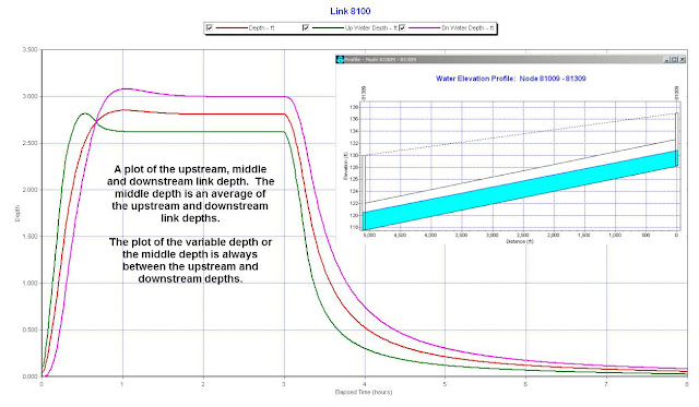
Three Depths in a Link in SWMM 5

Note: An explanation of the three depths in a Link in SWMM 5 and a plot of the upstream, middle and downstream link depth. The middle depth is an average of the upstream and downstream link depths. The plot of the variable depth or the middle depth is always between the upstream and downstream depths. All three depths are used in the computation of the St. Venant Flow in SWMM 5. The upstream area is a function of the upstream depth and the downstream area is a function of the downstream depth.
The dq4 term in dynamic.c uses the area upstream (a1) and area downstream (a2), the midpoint velocity, the sigma factor (a function of the link Froude number), the link length and the time step or
dq4 = Time Step * Velocity * Velocity * (a2 – a1) / Link Length * Sigma
the dq3 term in dynamic.c uses the current midpoint area (a function of the midpoint depth), the sigma factor and the midpoint velocity
dq3 = 2 * Velocity * ( Amid(current iteration) – Amid (last time step) * Sigma

Time Base is T + T*K from the Time(T) and Storage (K) values

Note: Each of the RDII UH’s has a base time for the convolution of the RDII from each UH. The Time Base is T + T*K from the Time(T) and Storage (K) values used in the RTK data. In this particular case:
· The Fast UH has a time base of 22 hours,
· The Medium UH has a time base of 430 hours, and
· The Slow UH has a time base of 4212 hours.
If this is altered as in the bottom image you can see the difference in the total RDII I&I Flow
· The Fast UH has a time base of 22 hours,
· The Medium UH has a time base of 36 hours, and
· The Slow UH has a time base of 52 hours.

H2OMAP-Sewer - FM Split Issue

Note: One method would be to add a duplicate Wet Well/Pump/Force Main set of links to pass the flow from the upstream Force Main to the two downstream Force Mains (FM). The pump should be fixed capacity to handle all of the split GM flows. In this particular example the flows are split 50/50 to links 25 and 35 after leaving the loading manhole 24.

Pumps and Force Mains in InfoSWMM

Note: A pump is modeled in InfoSWMM somewhat akin to InfoSewer. You have a Wetwell connected to a Pump which in turn is connected to a Force Main. You can decide wheter a pipe is a Force Main or a Gravity Main by using the Atribute Browser and selecting Yes for Force Main and entering a FM Roughness.

You can also use the PickAx tool in the Attibrute Browser to convert the node from a Manhole to a WetWell / Storage node.

RDII UH Storage Sensitivity

Note: The initial abstraction in the three RDII UH’s vary between 0 storage and maximum storage (Dmax). The speed of storage recovery is governed by the parameter Drec. You can see the sensitivity of this parameter in this graph of the UH Storage.

The Effect of the Hydrology Time Step on RDII Flow

Note: The wet hydrology time step and the report time step should be adjusted together to generate the smoothest RDII flow at your nodes. The three images show below show;

1. If you hydrology time step equals your rainfall time step then the RDII flow will have a step function appearance or your flows in this case will be constant for one hour or the rainfall interval,

2. If you choose a smaller hydrology time step then the flows will be smoother (2^nd image), but

3. If the report time step is much less than the hydrology time step then the flows will still be stepwise linear for the hydrology time step size.

When picking a hydrology time step for continuous simulation you should probably pick a value of about 5 minutes so that the generated flows are smooth but not so small that a lot of time is used in the RDIi convolution process to generate the 3 units hydrographs for RDII.

See and download the full gallery on posterous

Utilities/Locate/Element in InfoSWMM

You can use the command Utilities/Locate/Element to search for a number or string using Contains

 You will have to pick Contains each time.

SWMM 5 Related Websites

MY BLOG LIST

• 
  SWMM 5 or SWMM 5.0 Blog

  How to Use the SWMM 5 Excel Tool with InfoSewer CSV Files - How to Use the SWMM 5 Excel Tool with InfoSewer CSV Files 1. Export Link and Manholes in InfoSewer for your current Scenario to CSV files, 2. Set up the ...
  

  4 minutes ago
• 
  The South Florida Watershed Journal

  

  Belgian potato chips? - What’s your favorite flavor of chips? Interestingly, both the potato and the term barbecue are indigenous to the Americas While not exactly a watershed-rel...
  

  13 hours ago
• 
  Innovyze Blog

  2D meshing – Avoiding small elements (and why this is so important) - When generating a 2D mesh in Innovyze products (such as InfoWorks ICM, CS 2D and InfoSWMM 2D) it is very important to avoid small mesh elements, as just on...
  

  3 days ago
• SWMM5

  Increase in heavy rainfalls over past 60 years in upper Midwest, US - Increase in heavy rainfalls over past 60 years in upper Midwest, US http://www.sciencedaily.com/releases/2013/03/130313182312.htm March 14, 2013 Mar. 13...
  

  4 months ago
• 
  SWMM5 - Stormwater Management Model - SWMM 5, InfoSWMM, H20MAP SWMM, InfoSewer for Water Quality,Hydrology, Hydraulics

Conduit Lengthening in SWMM 5

Conduit Lengthening in SWMM 5
If you use the conduit lengthening option in SWMM 5 then your short conduits will be lengthened based on the CFL or explicit time step criterion. Any conduits in which the Length Factor or the courant time step link length over the original length is greater than 1 will be lengthened and will have its roughness lowered so that the conduit is hydraulically the same at full conduit depth. The full area, full width and full hydraulic radius stay the same in the modified link – only the length, slope and roughness are altered.
Length Factor = (Wave Celerity + Full Depth Velocity) * Time Step / Conduit Length, and for those links in which the Length Factor is greater than 1
New Roughness = Old Roughness / (Length Factor) ^1/2
New Slope = Old Slope / Length Factor
A few metric's for showing how this option has altered the network are shown in the figure below:
1. The most important is the increase in Network full volume as you never want to drastically alter the volume of your network,
2. The number of conduits modified along with the new mean slope (lower) and the new total conduit length are important indicators,
3. The mean wave celerity, full flow velocity and courant time step mean give the user some idea of the optimal time step for the simulation.

SWMM 5 Flooding Volumes for Ponding and Without Ponding

SWMM 5 Flooding Volumes for Ponding and Without Ponding

No Ponded Area for a Flooded Node

Ponded Area for a Flooded Node

Mud Flow in SWMM 5

Comment: A method to model Mud flow and other Non Newtonian Fluids in a modified SWMM 5.  You will have to modify the code as described in the link to actually model mud flow. Link Here

LPS Output Units when the Inflow is CMS

LPS Output Units when the Inflow is CMS

1. The inflow time series is in units of CMS,
2. If you set the internal units to LPS in Run Manager,
3. Set the output units to LPS in Output Unit Manager,
4. Add a Scale multiplier of 1000 in the Inflows DB Table then
The inflows do not have to be altered, the internal model flows will LPS, the velocity will be m/s with 6 decimal places in the RPT file and the flows will be LPS with 3 decimal places in the RPT file.

Opening and Closing an Orifice with a Time Series Setting

Opening and Closing an Orifice with a Time series Setting

An example of RTC rules in SWMM 5

The Three Flows in SWMM 5 for a Link

The Three Flows in SWMM 5 for a Link
There are actually three flows computed or used for a link in SWMM 5:
1. The St. Venant Flow equation flow
2. The Upstream Normal Flow Manning’s equation based on the link roughness, slope, upstream cross sectional area and upstream hydraulic Radius,
3. The flow actually used in the model which is either the flow computed from St. Venant or Manning’s equation
The following three links shows how this works in a real model:
· Link 8040 almost always uses the St. Venant Equation because it is dominated by backwater and surcharge
· Link 8100 almost always uses Manning’s equation except at the beginning and end of the simulation,
· Link 1600 is an adverse slope link and it mainly uses the St. Venant equation.
· Flow = the flow actually used during the simulation
· Qdynamic = the flow computed from the St. Venant Equation
· QNormUp = Flow based on Manning's equation at the upstream end of the link.
· QNormDown = Flow based on Manning's equation at the downstream end of the link.


Link 8100 almost always uses Manning’s equation except at the beginning and end of the simulation. The beginning and end of the simulation is when the non linear terms dominant.

Orifice Open and Close Speed and the Target Setting in SWMM 5

Orifice Open and Close Speed and the Target Setting
In SWMM 5 there is an orifice parameter called setting which opens or closes the orifice opening by modifying the depth of the orifice. The setting is based either on a RTC rule of the orifice or the Flap Gate condition of the orifice and can be between 0 and 1. Closed is 0; Open is 1. The difference is that the target setting is what the setting should be based on the condition of the Flap Gate or the RTC Rules and the setting is the value actually used in the model.
The open and close speed of the orifice modifies the orifice setting by changing the orifice setting based on the open and closing speed using the equation:
New Orifice Setting = Old Orifice Setting + (Target Setting – Orifice Setting) * Time Step / Orifice Open and Close Speed
If your target setting and the current orifice setting are both 1 or 0 then the orifice Open and Close option does not change the orifice setting. New Setting equals Old Setting in that case. If the target and setting are out of phase then the Open and Close Option will function correctly. For example, if the Open and Close Speed is 1 hour then the orifice setting will open and close in a one hour period. The table shown below shows how the orifice setting changes as a function of the speed and the difference between the target and orifice settings. The setting starts out open but the target says closed – the orifice then closes over a 1 hour period. At one hour the target setting is 1 and the orifice will then open over a one hour period.
Table - Link OR1@82309b-15009b
Setting Target
Days Hours
0 00:00:00 1.00 0.00
0 00:15:00 0.74 0.00
0 00:30:00 0.50 0.00
0 00:45:00 0.25 0.00
0 01:00:00 0.00 0.00
0 01:15:00 0.25 1.00
0 01:30:00 0.50 1.00
0 01:45:00 0.75 1.00
0 02:00:00 1.00 1.00
0 02:15:00 0.75 0.00
0 02:30:00 0.50 0.00
0 02:45:00 0.25 0.00
0 03:00:00 0.00 0.00
0 03:15:00 0.00 0.00
0 03:30:00 0.00 0.00
0 03:45:00 0.00 0.00

Example rule for the opening and closing of the orifice

Here is an example Real Time Control (RTC) rule for the opening and closing of an orifice.
RULE Orifice1
IF SIMULATION CLOCKTIME >= 01:00:00
AND SIMULATION CLOCKTIME <= 2:00:00
THEN ORIFICE OR1@82309b-15009b SETTING = 1
ELSE ORIFICE OR1@82309b-15009b SETTING = 0
PRIORITY 1
; Opens up the orifice at hour 1 of the simulation

SWMM 5 Link Time Step Calculations

SWMM 5 Link Time Step Calculations

It you select the variable time step option in SWMM 5 then the program will compute the CFL time step for each link based on the ending system variables in the last time step based on the following steps. The smallest value of t is used for each time step but often the same small set of links will be the controlling time for the whole simulation. In the example shown below link 1570c is controlling the time step 83 percent of the time. The link time step is usually the controlling time step.

Two Steady State Options in InfoSWMM and H2OMap SWMM

Two Steady State Options in InfoSWMM

Graphical Representation of Results in InfoSWWM

If you are graphing from the attribute browser you are restricted to 24 hours.
If you are using the report manager then you select the graphing by changing the From and To dates.

SWMM 5 Interface Guide Tips for C Compilers

SWMM 5 Interface Guide Tips
SWMM 5 has a Interfacing guide on http://www.epa.gov/nrmrl/wswrd/wq/models/swmm/#Downloads for creating a VB, Delphi or command line C program to both run and printout some of the output file results from SWMM 5. The readme file is self explanatory in the file http://www.epa.gov/nrmrl/wswrd/wq/models/swmm/swmm5_iface.zip but here are a few tips for those of you who want to compile the InterFaceGuide C code in a Executable file for Windows.
1. The first step is to make a new console program in Visual Studio

2. The second step is to add the files swmm5.h, swmm5_iface.h, swmm5_iface.c, test.c to the project header and source files.
3. Next add the file swmm5.lib as an additional dependency along with the directory name.
4. If you want to save the .out and .rpt files then you must comment out the remove statements at the end of test.c

5. You need to make a batch file to both run and save the input and output files from SWMM 5,
6. The file swmm5.dll must be in the same directory as the created interface executable file,
7. It will help you see the intermediate output if you add a pause statement in the batch file to hold the fprintf statements on the screen for you to view.

Weather Underground to SWMM 5 Rainfall Time Series

Weather Underground is a site that provides excellent local weather information in the form of graphs, tables and csv files. You can use the data very easily in SWMM 5 by copying from Excel to a time series in SWMM 5. Here is the rainfall for a storm event in Tampa, Florida in September, 2010

Export from WeatherUnderground using the CSV File Export Option

The data imported from the csv file to Excel and after the text to columns tool is used looks like this in Excel. The data is now ready to be imported into SWMM 5 after the time column is adjusted to fall on even 5 minute intervals. In Excel you can use the formula @ROUND((B2)/"0:05:00",0)*"0:05:00" to round all of the time values to 5 minutes. If you do not do this step then you will have problems in SWMM 5 due to the rainfall interval not being equal to the defined raingage interval.

You will need to format the new rounded time as a time format for import into SWMM 5

Open up and make a new time series in SWMM 5 and then copy and paste the date, rounded time column and rainfall column into the SWMM 5 time series columns.

DWF Scale Factor in SWMM 5 for entering Population Data

I (and a few others) think a welcome change to the DWF dialog in SWMM 5 would be the addition of another scale factor to modify the average flow field.  The purpose of the scale factor would be to allow the users to enter the DWF contributing population * the various DWF patterns * the scale factor (in units of cfs/person or l/s/person) in the Inflows dialog.  Some users of SWMM 5 prefer to use population directly in the GUI rather than doing this calculation externally and entering either the flow in cfs or l/s.  An example of why this would be useful is a future conditions model in which the population either increases or decreased in the catchment.

InfoSwmm import / export capabilities

InfoSWMM can both import and export to shapefiles and other databases using the Import and Export Manager, GIS Gateway and CSV file import and export generator.

SWMM5 Routing Time Step Summary

SWMM5 Routing Time Step Summary

This table is a summary of the iterations, times steps and amount of node and link bypasssing that occurs during a SWMM 5 simulation. It is listed in the text output file or the .rpt file of SWMM 5 which the file shown when you use the Report/Status command.

The minimum time step is the smallest time step used during the simulation.

The average time step is the mean time step used during the simulation.

The maximum time step is the maximum time used during the simulation.

The percent in steady state is the percent of the total simulation time spent in steady state during the simulation.

The average iterations per time step is the total number of iterations during the simulation divided by the total number of time steps or step count in this table. This will range between 2 and 4 iterations as SWMM 5.0.018 has a minimum of 2 and and a maximum of 4 iterations.

The Step count is the total number of time steps during the simulation.

The percent of bypassed links are the link flows that are NOT computed between time step iteration 2 and 4 because both the upstream and downstream node depths are converged in the current time step.

The percent of bypassed nodes are those nodes that have been converged between time step iteration 2 and 4. The node depth is still calculated, however, between iterations 2 and 4 as long as the whole time step is not considered converged.

Explicit Iteration Hydraulic Computation and Implicit Time Step Hydraulic Computations in SWMM 5

Explicit Iteration Hydraulic Computation and Implicit Time Step Hydraulic Computations in SWMM 5

The dynamic wave solution in SWMM 5 and InfoSWMM uses an interlocking explicit iteration in an overall time step implicit calculation of the node depths and link flows. The node depths and links flows are computed based on the last iteration values for 2 to 4 iterations. It explicitly calculates the node depths and link flows at each iteration based on the last iteration value but uses an underrelaxation or Gauss-Seidel method averaging to compute the final new iteration values. The underrelaxation method averages the last iteration value and the current iteration estimate to calculate the final iteration node depth and links flow.

At each time step this is the sequence of computations:

1. The time step is based on the Courant–Friedrichs–Lewy (CFL) condition for the most restrictive link (the CFL condition is based on the link length, current depth and current velocity),

2.Link flows and node depths are calculated at the 1^st iteration based on the last time steps flows and depths,

3. The new iterations link flow and node depths are calculated by averaging the node depths and link flows found in step 2 with the original iteration node depths and link flows,

4. The iteration process continues for at least 2 iterations for all nodes and links,

5. The iteration process may stop after 2 iterations for those links in which the upstream and downstream node depths have converged,

6. The upstream or downstream node is considered converged when the absolute depth difference between iterations is less than 0.005 feet,

7. The maximum number of iterations for all nodes and links is set to 4.

8. Once the number of iterations has reached 4 or all nodes and links are converged the time step calculations are considered finished and the program moves on to a new time step.

9. The image shown below shows how the node continuity equation is solved for each iteration but the link combined continuity and momentum equation is calculated for either 2, 3 or 4 iterations depending on the upstream and downstream node convergence of the link.

Steady State Option in SWMM 5

The skip steady state periods uses the last computed flows in the conveyance system instead of computing new flows. In the sample graphs you can see where the change in lateral flow is below 0.05 cfs (the blue arrow in the second image). The network solution used the steady flows about 27 percent of the time. The time step summary in the text output file tells you how often the model was in steady state.

Skip Steady State Periods
Checking this option will make the simulation use the most recently computed conveyance system flows during a steady state period instead of computing a new flow routing solution. A time step is considered to be in steady state if the change in external inflow at each node is below 0.5 cfs and the relative difference between total system inflow and outflow is below 5%.

Lead and Lag Pump Options in SWMM 5

Introduction: If you have a lead and lag pump connecting the same upstream and downstream nodes the normal behavior for the two pumps is to have the the lead pump turn on first followed by the lag pump. The turn on and turn off depths for the pumps determine when the pumps turn of. The pump will work as a simple lead and lag pump based on a wet well elevation without any real time controls.

If you want to add real time controls (RTC) to the lead and lag pumps you can add more sophisticated controls. For example, if you wanted to turn on and off the lead pump at successive time steps then you can add these RTC rules

; New Real Time Control (RTC) Rules

RULE RULE-1

IF PUMP LEAD_PUMP STATUS = ON

AND PUMP LAG_PUMP STATUS = ON

THEN PUMP LEAD_PUMP STATUS = OFF

PRIORITY 1.000000

RULE RULE-2

IF PUMP LEAD_PUMP STATUS = OFF

AND PUMP LAG_PUMP STATUS = ON

THEN PUMP LEAD_PUMP STATUS = ON

PRIORITY 1.000000

RULE RULE-3

IF PUMP LEAD_PUMP STATUS = OFF

AND PUMP LAG_PUMP STATUS = ON

THEN PUMP LEAD_PUMP STATUS = ON

PRIORITY 1.000000

If you want to add a pattern of 2 time steps and 1 time step off for both pumps then you can add this RTC new rule to control the lag pump:

RULE RULE-4

IF PUMP LEAD_PUMP STATUS = OFF

AND PUMP LAG_PUMP STATUS = ON

THEN PUMP LAG_PUMP STATUS = OFF

PRIORITY 1.000000

SWMM 5 Link Iterations

These three graphs show how the number of iterations to solve the St. Venant equation in SWMM 5 changes during the course of the simulation based on rapidly changing inflow, steady inflow and decreasing inflow. This example allows up to ten iterations and a tighter head tolerance to better illustrate how the number of iterations increase at the beginning of the simulation and during rapid inflow. Normally, in SWMM 5 the number of iterations will be between a minimum of 2 and a maximum of 4 iterations.

In the first graph the outflow is in blue and the number of iterations at each time step is shown in red. In the second graph the bubble size is based on the number of iterations and the y axis is outflow of the network. The third graph shows the number of iterations used at each link in the model at a particular time step. The more the flow changes the more iterations are needed to keep the flow in balance.

SWMM5 Bubble Plot of Continuity Error

The overall continuity error at any time during the simulation is simply the total inflow minus the total outflow. The total inflow is the dry weather, wet weather, groundwater, I&I inflow, external inflow and the initial network storage. The total outflow is the amount of surface flooding, outfall flow, reacted flow and the final storage.

Continuity error = Total Inflow - Total Outflow

The continuity error can be variable over time as this graph of the total inflow, total outflow and continuity error over time shows for the classic extran example from SWMM 3 and SWMM 4. The continuity error can be negative or positive at each saved time step and it tends to balance out over time. As you can imagine depending on how long the simulation lasts the continuity error may be much greater than zero. If you can the simulation to dry weather flow is reached in the sanitary network or the stormwater network has drained the continuity error will be better. You can see that the CE increases at the beginning of the simulation, continues on and then goes to zero CE when the system drains.

If we look at a bubble chart of the continuity error over time (with the bubble size the continuity error) and the y axis the Total Inflow to the network you can see how continuity error increases and then decreases over time. The white bubbles are negative continuity error points.

SWMM 5 Conduit Lengthening

If you use the conduit lengthening option under the dynamic tab the shorter lengths will be lengthened internally during the simulation and the results will be a smoother.