Force Main Friction Loss in SWMM 5

Subject:  Force Main Friction Loss in SWMM 5

You can model Force Mains in SWMM 5 using either Darcy Weisbach or Hazen Williams as the full pipe friction loss method (see Figure 1 for the internal defintion of full flow).   No matter which method you use for full flow the  program will use Manning’s equation to calculate the loss in the link when the link is not full (see Figure 2 for the equations used for calculating the friction loss – variable dq1 in SWMM 5).  Force Main Friction Loss in SWMM 5.

Figure 1.  How the full pipe condition is defined in SWMM 5

Figure 2:  Friction equations used in SWMM 5 for a Force Main.

Figure 3:  Regions of Friction loss equations in SWMM 5.

Capacity Limited Links in SWMM 5

Subject: Capacity Limited Links in SWMM 5

The table in the text report file of SWMM 5 called “Conduit Surcharge Summary” has a column entitled “Hours Capacity Limited” Here is how a link is defined as Capacity Limited in SWMM 5. Two factors have to be present:

1. The upstream end of the link has to be full and

2. The HGL Slope has to be greater than the Slope of the Link

What is the Area of a Node in SWMM 5?

Subject: What is the Area of a Node in SWMM 5?

The minimum area of a node is the default area of the node, which is the user defined minimum surface area or 12.566 square feet if the user does not define the surface area of the node. The surface area of a node is usually the half of the surface area of all of the connecting conduits but if the link is dry then the sum of all of the surface areas may be less than the default surface area. If you look at a scatter plot of the area versus the depth then you will see that it always has the minimum surface area.

What is Node Convergence in SWMM 5?

Subject: What is Node Convergence in SWMM 5?

If a link has converged within two iterations then the hydraulic computations will be bypassed for the link in new iterations. A link is deemed converged if BOTH the upstream and downstream node depth has converged between successive iterations as long as two iterations have occurred during the time step. The nodes are considered converged if the depths between successive iterations is less than the stop tolerance of the program (the default stop tolerance is 0.005 feet). The new node depths are ALWAYS computed for each iteration but the links connected to the converged nodes may bypass computations and save on simulation time. Note: If the nodes ever become non converged after 2 iterations then the link flows will be computed.

What is Link Bypass in SWMM 5?

Subject: What is Link Bypass in SWMM 5?

If a link has converged within two iterations then the hydraulic computations will be bypassed for new iterations. A link is deemed converged if BOTH the upstream and downstream nodes depth has converged between successive iterations as long as two iterations have occurred during the time step. This is simulation savings step as it my eliminate up to 75 percent of the computational time in a SWMM 5 simulation. The image below shows that for some links the flow in the link is converged within 2 iterations whereas for others it may take 3 or 4 iterations. Overall, 37 percent of the link computations are bypassed during the simulation of this particular hydraulic network.

Time Step Critical Elements in SWMM 5

Subject: Time Step Critical Elements in SWMM 5

The time step critical elements in the SWMM 5 report text output file tells you which elements were controlling the time step during the simulation. If no element was controlling the time step then the program will just use the maximum time step. For example, if the maximum time step was 10 seconds and the average time step was 9.8 then only a few time steps were set by a link or node that needed a smaller than maximum time step (Figure 1). If the maximum time step for the same simulation was 30 seconds then many links and nodes will set the time step (Figure 2).

Figure 1. Most of the time the simulation used the maximum time step of 10 seconds so only a few links were time step critical.

Figure 2. Most of the time the simulation used less than the maximum time step of 30 seconds so many links were time step critical.

Pump Power Usage in SWMM 5

Subject: Pump Power Usage in SWMM 5

The pumping summary table (Figure 1) includes a column that tells the user how much power was consumed by the pump in kilowatts by the head loss or head gain of the water flowing through the pump. The power usage equations are shown in Figure 2.

Figure 1. Pump Summary Table in SWMM 5.0.021

Figure 2. Pump Power Equations in SWMM in which dt is the time step.

Non Linear Term in the Saint Venant Equation of SWMM 5

Non Linear Term in the Saint Venant Equation of SWMM 5The flow equation has six components that have to be in balance at each time step:

1. The unsteady flow term or dQ/dt

2. The friction loss term (normally based on Manning's equation except for full force mains),

3. The bed slope term or dz/dx

4. The water surface slope term or dy/dx,

5. The non linear term or d(Q^2/A)/dx and

6. The entrance, exit and other loss terms.

All of these terms have to add up to zero at each time step. If the water surface slope becomes zero or negative then the only way the equation can be balanced is for the flow to decrease. If the spike is due to a change in the downstream head versus the upstream head then typically you will a dip in the flow graph as the water surface slope term becomes flat or negative, followed by a rise in the flow as the upstream head increases versus the downstream head.

You get more than the normal flow based on the head difference because in addition to the head difference you also get a push from the non linear terms or dq3 and dq4 in this graph.

If you use the Keep Inertial term option then you use all 5 terms at all times, if you use the Dampen option you use all five terms until the Froude number of the link greater than 1 and then you do not use terms dq3 and dq4, if you use the Ignore option then the dq3 and dq4 terms are not used at all for the calculation of the flow in the link.

The number of Hydraulic Iterations in Various Versions of SWMM 5

Subject: The number of Hydraulic Iterations in Various Versions of SWMM 5.

The maximum number of iterations was 4 before SWMM 5.0.021 and 8 iterations after SWMM 5.0.021. In InfoSWMM and H2OMAP SWMM you can have a a minimum of 2 iterations or a maximum of 8 iterations for compatibility to SWMM 5 and backwards compatibly with your earlier InfoSWMM models.

.

Time Step Selection in SWMM 5

Subject: Time Step Selection in SWMM 5
1^st The time step you use in SWMM 5 is controlled from the top by the rainfall interval (Figure 1):
1. All of your time steps should be less than the rainfall interval,
2. The hydrology time step should be less than or equal to the smallest raingage rainfall interval in your network,
3. The hydraulic time step should be less than or equal to the hydrology time step and should be based on the hydraulic needs of the your network. Short length links, pump and weirs may require a smaller maximum hydraulic time step.
2^nd The report time step controls what you see in the graphics output of SWMM 5. If you see a large difference between that you see in the graphics output and the report text file it is because you have a large difference between the report time step and the average time step used during the simulation.
Solution: If there is a large discrepancy in the graphics and report text file then the best solution is to reduce the maximum time hydraulic time step so it is closer to the average time step and also to make the report time step closer to the Maximum time step (Figure 2).

Figure 1: Relationship between the rainfall, hydrology and hydraulic time steps.

Figure 2: Relationship between the minimum, average and maximum simulation time steps and the report time step.

Pump Priorities in SWMM 5

Subject: Pump Priorities in SWMM 5

The Startup and Shutoff depths are evaluated 1^st followed by any Control Rules. The priority value is just to decide between two or more control rules that are both active at the current time step. The rule with the highest priority will be used or in the case of two rules with the same priority the last control rule evaluated will be used during the current time step.

Node Surcharge Summary in SWMM 5

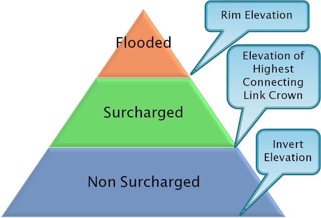
In SWMM 5 (Storm Water Management Model), surcharging refers to a condition where water levels rise above the highest point, or crown, of the conduits (pipes) in the drainage network. This situation usually occurs when the system's capacity is exceeded due to high levels of stormwater or wastewater inflow.

The SWMM 5 report file (RPT file) includes a Node Surcharge Summary Table, which provides crucial details about the duration and extent of these surcharging events.

Node Surcharging:

A node is a point in the network where pipes connect. Surcharging can occur at a node in the following conditions:

1. If the node cannot store additional water (i.e., it cannot 'pond') and the water depth at the node exceeds the crown elevation of the highest pipe connected to that node.

2. If the node can store additional water (it can 'pond'), surcharging occurs when the water depth exceeds the crown elevation of the highest pipe connected to the node but remains below the full depth of the node.

Essentially, surcharging happens when the system cannot accommodate the excess water, leading to water levels rising above the pipe's topmost part but not yet reaching the full depth of the node.

Node Flooding:

Node flooding is a more extreme event that occurs when the water surface level reaches or surpasses the rim elevation of the node. This situation means that the water is spilling out of the system, potentially leading to surface flooding.

Node Surcharge Summary Table (Figure 1)

This table in the RPT file presents a summary of the surcharging events at each node, including the duration of surcharging.

Definition of Surcharging at a Node (Figure 2)

This figure would typically show a diagram or explanation illustrating the conditions under which a node is considered to be surcharging, visually demonstrating the situations described above.

Definition of the Height above Crown and Depth below Rim (Figure 3)

This figure would likely provide definitions or illustrations explaining the 'Height above Crown' and 'Depth below Rim' columns in the Node Surcharge Summary Table. 'Height above Crown' refers to how much higher the water level is compared to the crown of the highest pipe, while 'Depth below Rim' refers to the difference between the water level and the full depth of the node.

These details allow engineers to understand the behavior of the drainage system under various flow conditions and inform necessary adjustments or improvements to manage stormwater effectively.

Swamee and Jain approximation to the Colebrook-White equation in SWMM 5

Note: There is a function called ForceMain in SWMM5/InfoSWMM whose purpose is to compute the Darcy-Weisbach friction factor for a force main using the Swamee and Jain approximation to the Colebrook-White equation.
f = forcemain_getFricFactor(xsect.rBot, d/4.0, 1.0e12);
return sqrt(f/185.0) * pow(d, (1./6.));
double forcemain_getFricFactor(double e, double hrad, double re)
//// Input: e = roughness height (ft)
// hrad = hydraulic radius (ft)
// re = Reynolds number
// Output: returns a Darcy-Weisbach friction factor
// Purpose: computes the Darcy-Weisbach friction factor for a force main
// using the Swamee and Jain approximation to the Colebrook-White equation.
{ double f;
if ( re < 10.0 ) re = 10.0;
if ( re <= 2000.0 ) f = 64.0 / re;
else if ( re < 4000.0 )
{ f = forcemain_getFricFactor(e, hrad, 4000.0);
f = 0.032 + (f - 0.032) * ( re - 2000.0) / 2000.0; }
else { f = e/3.7/(4.0*hrad);
if ( re < 1.0e10 ) f += 5.74/pow(re, 0.9);
f = log10(f);
f = 0.25 / f / f; }
return f;}

From http://en.wikipedia.org/wiki/Darcy_friction_factor_formulae
http://www.swmm2000.com/profiles/blogs/swamee-and-jain-approximation

Link Surcharging Definitions in SWMM 5

Subject: Link Surcharging Definitions in SWMM 5

The report or RPT text output file of SWMM 5 contains a table that lists the Surcharged Conduits during the simulation (Figure 1).
The 5 columns in the table are:

1. Hours Both Ends Surcharged
2. Hours Upstream End Surcharged
3. Hours Downstream End Surcharged
4. Hours Above Full Normal Flow
5. Hours Capacity Limited

.the five columns are defined in Figure 2. Notice that if the midpoint of the link is full then the link and both end of the link are considered to be surcharged. If the midpoint is NOT full then the cross sectional area of the ends of the link determine wheter the ends of the link are considered surcharged. The end of a link can be considered surcharged based on either the depth at the midpoint or the cross sectional area at the end of the link.

Figure 1: The SWMM 5 Conduit Surcharge Table

Figure 2: The SWMM 5 Conduit Surcharge Table Definitions, the numbers in the 3^rd column correspond to the columns in the Conduit Surcharge Table.

PID Control in SWMM 5 for an Orifice

Click here to download:

extran_pid_3_master.inp (47 KB)

Subject: PID Control in SWMM 5 for an Orifice

The blog http://swmm5.blogspot.com/2010/12/pid-control-in-swmm-5-for-type-3-pump.htmldescribes the Function getPIDSetting which returns the PID setting at each time step. The PID parameter set contains three values -- a proportional gain coefficient, an integral time (in minutes), and a derivative time (in minutes) which are kp, ki and kd, respectively. More about the theory of PID controllers can be found at http://en.wikipedia.org/wiki/PID_controller.

Here is an example PID Rule that will keep the node depth at 5 feet in a SWMM 5 model by changing the Orifice Setting. The Orifice setting opens and closes the orifice over time. The example file is attached in this blog. In this particular example, you can reduce the oscillations about the 5 foot rule level by lowering the integral time and derivative time coefficients in the PID control rule. An important note is that for Weirs and Orifices the setting is bounded to be between 0 and 1. If the Orifice or Weir cannot handle the upstream node inflow then the PID control will not be able to meet the depth goal in the node. For example, in the example file, an orifice depth of 2 feet is not enough to meet the upstream node depth goal of 5 feet but a 3 foot orifice is large enough for the PID control to meet its stated goal of 5 feet. The PID control will only work if the link doing the controller has enough flow and depth flexibility.

RULE PID_Orifice

; the PID controller adjusts the orifice opening to have a

; depth of 3 feet in Node 82309b

IF NODE 82309b DEPTH <> 5

THEN ORIFICE OR1@82309b-15009b SETTING = PID 10 -0.01 -0.01

; kp ki kd

PRIORITY 1

PID Control in SWMM 5 for a Weir

Subject: PID Control in SWMM 5 for a Weir

The blog http://swmm5.blogspot.com/2010/12/pid-control-in-swmm-5-for-type-3-pump.html describes theFunction getPIDSetting which returns the PID setting at each time step. The PID parameter set contains three values -- a proportional gain coefficient, an integral time (in minutes), and a derivative time (in minutes) which are kp, ki and kd, respectively. More about the theory of PID controllers can be found at http://en.wikipedia.org/wiki/PID_controller.

Here is an example PID Rule that will keep the node depth at 3 feet in a SWMM 5 model by changing the Weir Setting. The example file is attached in this blog. In this particular example, you can reduce the oscillations about the 3 foot rule level by lowering the integral time and derivative time coefficients in the PID control rule.

RULE PID_Weir
; the PID controller adjusts the weir height to have a
; depth of 3 feet in Node 82309e
IF NODE 82309c DEPTH <> 3
THEN WEIR WEIR1@82309c-15009c SETTING = PID 10 -.01 -.01
; kp ki kd
PRIORITY 1

PID Control in SWMM 5 for a Type 3 Pump

Subject: PID Control in SWMM 5 for a Type 3 Pump

Figure 2 shows the code in Function getPIDSetting which returns the PID setting at each time step. The PID parameter set defines the degree of control. The PID parameter set contains three values -- a proportional gain coefficient, an integral time (in minutes), and a derivative time (in minutes) which are kp, ki and kd, respectively. More about the theory of PID controllers can be found at http://en.wikipedia.org/wiki/PID_controllerand shown in Figure 3.
Here is an example PID Rule that will keep the node depth at 3 feet in a SWMM 5 model.
RULE PID1
; the PID controller adjusts the flow in the pump to have a
; depth of 3 feet in Node 82309e
IF NODE 82309e DEPTH <> 3
THEN PUMP PUMP1@82309e-15009e SETTING = PID 10 -1 -1
; kp ki kd
PRIORITY 1


Figure 1: SWMM 5.0.021 Simulation Results

Figure 2: Source code for getPIDSetting in SWMM 5.0.021

Figure 3: Image source for the Block Diagram of a PID Controller Pid-feedback-nct-int-correct.png

Total Surcharge Time vs Total Time Above Rim Elevation in InfoSWMM

Subject: Total Time Above Rim Elevation at a Node
1. Total Surcharge Time is the total time above the crown of the highest connecting pipe to a node.

2. Total Time Above Rim Elevation – this is the flooding time of the node and it includes flood time as well as ponding time. You can find this in the Junction Summary Report of InfoSWMM under the column Total Flood Time. The Total Flood Time is less than the Total Surcharge Time as the depth in the Node is higher.

1. A node is flooded if the node depth equals the node rim elevation – the flooded time is the total time excess flow coming out the top of the manhole,
2. A node is flooded if the node depth is above the rim elevation and you are using the Surface Ponding Option – the flooded time is the ponding time
3. A node is flooded if the node depth equals the node surchage elevation – the flooded time is the total time excess flow coming out the top of the surcharged manhole.

SWMM 5 Controls in Matrix Form

Subject: SWMM 5 Controls

IBM helps the City of Corpus Christi get smarter

IBM’s Guru Banavar discusses how Corpus Christi is getting smarter by tracking the city’s assets. In order to keep the citizens happy, you have to manage the city’s assets.

Wellington E Webb, the former mayor of Denver, Colorado, once said: “The 19th century was a century of empires, the 20th century was a century of nation states. The 21st century will be a century of cities.”

...

That’s why the cities need to be smarter. And to do this, each part of the infrastructure needs to be more intelligent. This means the cities need to start collecting data on everything including streets, bridges, parks, buildings, fire hydrants, water mains and storm water ditches. Link Here

Calibration Concepts from Serendipity

From the blog Serendipity as useful discussion on calibration

..ask what is the purpose of a climate model. The second half of the George Box quote is “…but some models are useful”. Climate models are tools that allow scientists to explore their current understanding of climate processes, to build and test theories, and to explore the consequences of those theories. In other words we’re dealing with three distinct systems:

We're dealing with relationships between three different systems

There does not need to be any clear relationship between the calculational system and the observational system – I didn’t include such a relationship in my diagram. For example, climate models can be run in configurations that don’t match the real world at all: e.g. a waterworld with no landmasses, or a world in which interesting things are varied: the tilt of the pole, the composition of the atmosphere, etc. These models are useful, and the experiments performed with them may be perfectly valid, even though they differ deliberately from the observational system.

What really matters is the relationship between the theoretical system and the observational system: in other words, how well does our current understanding (i.e. our theories) of climate explain the available observations (and of course the inverse: what additional observations might we make to help test our theories). When we ask questions about likely future climate changes, we’re not asking this question of the the calculational system, we’re asking it of the theoretical system; the models are just a convenient way of probing the theory to provide answers.

By the way, when I use the term theory, I mean it in exactly the way it’s used in throughout all sciences: a theory is the best current explanation of a given set of phenomena. The word “theory” doesn’t mean knowledge that is somehow more tentative than other forms of knowledge; a theory is actually the kind of knowledge that has the strongest epistemological basis of any kind of knowledge, because it is supported by the available evidence, and best explains that evidence. A theory might not be capable of providing quantitative predictions (but it’s good when it does), but it must have explanatory power.

More Here: http://www.easterbrook.ca/steve/?p=2032&cpage=1#comment-4945

I redid the above graphic in Powerpoint

In terms of SWMM 5 and other models let me paraphrase the above:

We're dealing with relationships between three different systems

There does not need to be any clear relationship between the calculational system and the observational system – I didn’t include such a relationship in my diagram. For example, hydrology/hydraulic models can be run in configurations that don’t match the real world at all: e.g. a watershed without detail or simple assumptions, or a watershed in which interesting things are varied: the modeling detail for catchment complexity, slope, overland path length, impervious connections, soil and infiltration detail and methodology. You can also leave out important components such as ground water and water quality. These models are useful, and the experiments performed with them may be perfectly valid, even though they differ deliberately from the observational system.

What really matters is the relationship between the theoretical system and the observational system: in other words, how well does our current understanding (i.e. our theories) of hydrology/hydraulics explain the available observations (and of course the inverse: what additional observations might we make to help test our theories). When we ask questions about likely future watershed changes, we’re not asking this question of the the calculational system, we’re asking it of the theoretical system; the models are just a convenient way of probing the theory to provide answers.

How to Decide on a Time Step in InfoSWMM

Note: How to Decide on a Time Step in InfoSWMM

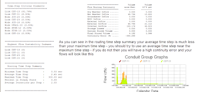
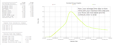
Step 1: Your first guess was 300 seconds which had a very large continuity and unstable links. If you look at the your average time step a good time step would be 10 seconds based on your average time step of 2.6 seconds.

Step 2: Run your model with a time step of 10 seconds and check the flows and the continuity error. In this case by using a maximum time step near the average time step you got rid of the continuity error and the unstable link flows.