The Pump summary table of SWMM5.0.022 and the Percent Time off Columns

Subject:  The Pump summary table of SWMM5.0.022 and the Percent Time off Columns

The pump summary table at the end of the SWMM 5 report file has two columns for the time off the pump curve BUT the two columns are only informative if the pump is a type 4pump.  If the pump type is 1, 2 or 3 then the low column is always 0 and when the volume, depth or head is either below the lowest point in the point curve or above the highest point in the pump curve the pump summary table lists the time off either low or high in the High column.

xMin is  the 1^st point in the pump curve for either volume, depth, head or depth, respectively for pump1, pump2, pump3 and pump4 type pumps

xMax is the last point in the pump curve for either volume, depth, head or depth, respectively for pump1, pump2, pump3 and pump4 type pumps

Average Residence time in InfoSWMM and H2OMAP SWMM

Subject:  Average Residence time in InfoSWMM and H2OMAP SWMM

Here is one way to estimate the residence time:

1.       Plot the System Outflow and Storage in the InfoSWMM Report Manager

2.       Click on the Report Button and copy the Outflow and Storage Time Series

3.       Paste to  Excel

4.       Calculate the Residence time as Storage / Outflow and Graph

5.       You will have an understanding of the residence time in your network

6.       If you have a dry weather flow then a hot start file will give a better estimate at the start of the simulation 

An Example of the Importance of the Term DQ4 in the SWMM 5 St Venant Solution

Subject:   An Example of the Importance of the Term DQ4 in the SWMM 5 St Venant Solution

The four terms are are used in the new flow for a time step of Qnew:

Qnew = (Qold – dq2 + dq3 + dq4) / ( 1 + dq1)

when the force main or gravity main is full dq3 and dq4 are zero and  Qnew = (Qold – dq2) / ( 1 + dq1)

The dq4 term in dynamic.c uses the area upstream (a1) and area downstream (a2), the midpoint velocity, the sigma factor (a function of the link Froude number), the link length and the time step or

dq4 = Time Step * Velocity * Velocity * (a2 – a1) / Link Length * Sigma

where Sigma is a function of the Froude Number and the Keep, Dampen and Ignore Inertial Term Options.  Keep sets Sigma to 1 always and Dampen set Sigma based on the Froude number, Ignore sets Sigma to 0 all  of the time during the simulation.

The value of dq4 increases when there is a significant difference in the cross sectional  area of the downstream end of the link and the upstream end of the link.  In this  example, the downstream storage node causes a backflow in the link.   The flow may look unstable in the link  flow time series but the change in flow is simply due to the water sloshing back and forth.  There is not continuity error as the term dq4 keeps the water in the link  in balance.

Use the SWMM 5 Scatter Graph to show the Pump Curve used during the Simulation

Subject:  Use the SWMM 5 Scatter Graph to show the Pump Curve used during the Simulation

You can use a scatter graph to show the relationship between the pump during the simulation and the Storage Depth.   If the pump is on the curve based on the pump summary table then the scatter graph should  look like the pump curve.  The pump summary table in the  SWMM 5 RPT also shows you the time off the pump curve low and high. 

How to Import the SWMM 5 Report File as a Layer in infoSWMM

Subject:  How to Import the SWMM 5 Report File as a Layer in infoSWMM

The idea of this blog of note is to show how one may extract information from the SWMM 5 or InfoSWMM RPT file and import the Excel  File as a feature in InfoSWMM.  This blog has an example Excel file to illustrate the linkage. The steps are:

Step 1:  Copy the whole row  from Conduit Summary from the InfoSWMM Browser

Step 2:  Add the two columns length and  slope from the Link Summary Table and the InfoSWMM Browser

Step 3:  You need a few calculations based on the table values from SWMM 5 to estimate the CFL  time steps in the .

Step 4:   Add the Excel Spreadsheet as a layer in InfoSWMM – the Named Range should be added to insure valid numbers and not Nulls after the join

Step 5:  You can now plot the CFL Time Step for the Links using the Layer Properties command in Arc Map

  

Step 1:  Copy the whole row  from Conduit Summary

Step 2:  Add the two columns length and  slope from the Link Summary Table

Step 3:  You need a few calculations based on the table values from SWMM 5 to estimate the CFL  time steps.

The CFL Step      = Length / (Full  Velocity + (Gravity * Full Depth)^0.5)

Full Velocity        = Full Flow / Full  Area

You also need to create a Name A Range for you data so that the data does not show up as Nulls

Step 4:  Add the Excel Spreadsheet as a layer in InfoSWMM – the Named Range should be added

Step 4:  Join the Excel  Table to the InfoSWMM Conduit Feature Layer

Step 5:  You can now plot the CFL Time Step for the Links using the Layer Properties command in Arc Map

How to Approximate a Timer in the RTC Rules of SWMM 5

Subject:   How to Approximate a Timer in the RTC Rules of SWMM 5

SWMM 5 does not have a explicit timer in its Real Time Control (RTC) rules but you can approximate it by using a Control Curve as in the attached example model.  The Control Curve will modify the setting of the Weir by the Inflow to the Storage node.  You can have normal weir flow settings based on the invert elevation of the weir and the Surface node water surface elevation but in addition you can control the weir setting by:

1.   Closing the weir when the inflow is low,
2.   Closing the weir by staggered Storage node depth,
3.   Opening the weir gradually when the inflow increases
4.   Closing the weir by a combination of Node Depth IF statements and Control Curve rules

For example, you can have the Weir Setting controlled the Node Depth,  Link Inflow and Node Inflow  simultaneously approximately with the depth and the inflow parameters closing the weir by proxy instead of by time since the closing.

The Importance of Viewing Results at the Proper Time Scale in SWMM5 and InfoSWMM Models

Subject:   The Importance of Viewing Results at the Proper Time Scale

In SWMM 5 when you are simulating rapidly changing flow – such as pump flows – it is important to  remember that you are only seeing the results of the simulation at your selected report time step.  Here is an example model with the same number of pump starts for all three simulations (318), the same  average time step during the simulation (10 seconds) but different report time steps.  The conception of the pump starts is totally different visually depending on the selected report time steps.  You should always compare the starts using the pump graphs and the pump summary table.    The percent utilized and the number of pump start ups tells you  the mean pump start length or in this case 153 seconds or 45.1 percent of 30 hours divided by 318 pump starts.

How to Make a Smaller Model out of a Large Model in InfoSWMM

Subject:   How to Make a Smaller Model out of a Large Model in InfoSWMM

InfoSWMM and H2OMAP SWMM will export only those ACTIVE elements to SWMM 5 as defined by the Facility Manager. 

You can use to feature to make smaller SWMM 5 models and then reimport the exported smaller SWMM 5 model back into a H2OMAP SWMM or InfoSWMM scenario.

How to Copy from a SWMM 5 Table to Excel

Subject:  How to Copy from a SWMM 5 Table to Excel 

Step 1. Highlight the rows you want to copy to Excel 

Step 2:  Use the Copy to Clipboard or Copy to File command 

Step 3:  Paste in Excel or open the exported text file  

How to Make a SWMM 5 Calibration File from InfoSWMM

Subject:  How to Make a SWMM 5 Calibration File from InfoSWMM 

1^st Step:  Graph a Link  in InfoSWMM using the Date /Time Format

2^nd Step:  Click on the Report Button and copy the 1^st two columns of data

3^rd Step:  Save the  copied columns to a data file, replace the semi colon and add the name of the link  to the top of the data file as shown below

4^th Step:  Connect the created calibration data file t o the SWMM 5 Calibration Data Link Flow Rate

5^th Step:  Run the  Simulation and you should see two  graphs on the screen for the designated link

RDII or Tri Triangular Unit Hydrograph in InfoSewer

Subject:  RDII or Tri Triangular Unit Hydrograph in InfoSewer

The RDII method in InfoSewer is similar to the RDII or RTK  method in  InfoSWMM with some differences.    The RTK data for triangles 1, 2 and 3 are defined in the Unit Hydrograph but instead of individual R values, the overall R is set and the Percent R1,  R2 and R3 are defined based on the total  R.  R3 is calculated internally as 100 – R1 – R2.   Each loading manhole with RDII flow has a total  area, a hyetograph and a Unit Hydrograph.  The hyetograph has to be set at multiples of the unithydrograph, so you can define the time or X columns with integers and then use the Block Edit command to change X to minutes by multiplying  by the Unit Hydrograph time (Figure 1).   You can use only one component if you set R1 or R2 to 100 percent or R3 to 100 percent by setting R1 and R2 to 0 percent (Figure 2).  The overall area of the Unit Hydrograph is divided amongst the loading manhole using the Subbasin Area (Figure 3).   The storm flows generated can be viewed using a Group Graph (Figure 4).

Figure 1.   Hyetograph Curve for the RDII Unit Hydrograph

Figure 2.  The Unit Hydrograph is defined for various values of R, R1,  R2, T1,  T2,  T3, K1,  K2 and  K3.

Figure 3.  The Unit Hydrograph and Hyetograph are tied to a particular loading manhole using a Subbasin Area.

Figure 4.  The Unit Hydrographs that are generated can be viewed using a Group loading Manhole Graph.  The R1, R2 and R3 have only one triangle.

 .

How InfoSWMM and H2oMAP SWMM Reads CUHP Hydrographs

Note:  The Colorado Urban Hydrograph Procedure (CHUP) 2010 version generates a SWMM 5 Inflows Files containing a time series of flow inflows for 1 to many nodes (Figure 4 and Figure 5).    The created Inflows file (Figure 2) can be imported intao InfoSWMM and H2MAP SWMM without any alteration by using the Files command in Run Manager (Figure 1) and graphed using the Output Manager of InfoSWMM and  H2OMAP SWMM (Figure 3).

Figure 1.  Location of Files Command in Run Manager

The inflows will be read  from the Inflows file, which has this format:

Figure 2.  Header format of the CUHP Exported Hydrograph File

InfoSWMM and H2oMAP SWMM will match the Node Names in the Inflows file to the network node names and import and interpolate the inflows based on the Inflows time step and your hydraulic time step to generate Lateral  Inflow Hydrographs

Figure 3.  InfoSWMM and H2OMAP SWMM Lateral  Inflow Hydrographs

Figure 4.  CHUP Inflows File Descrpiption in the CUHP manual.

Figure 5. Cover of CUHP 2005 User Manual from 2010

How to Find the Proportional loading to a link or manhole in InfoSewer

Subject:  How to Find the Proportional loading to a link  or manhole in InfoSewer

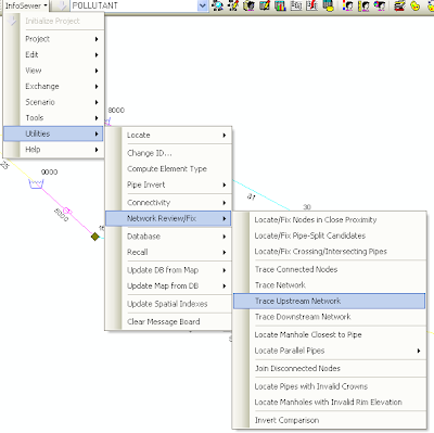
You can use the Upstream Trace tool in InfoSewer to find the upstream nodes and links from any link in InfoSewer.   Once you have the upstream traced network then assing the traced upstream nodes and links to the  domain.  Once you have the domain then these steps will allow you to calculate the proportion of flows from each upstream node and map the proportion using Map Display.

Step 1.  Use the Tool Trace Upstream Network to find and make a Domain out of the Traced upstream Network

Step 2.  The Traced Upstream Network

Step 3.  Use the created domain in Output Report Tabular Reports

Step 4.  Copy the ID and Total Flow from the Loading Manhole Report

Step 5.  Use the Domain in the DB Table Manhole Infomation

Step 6.  Create a new information field called Proportion for example

Step 7.  Map the new data field proportion using Map Display

Step 8.  Now you have a Map Display of the Proportional loading to a link  or manhole in InfoSewer

Step 9.  40 percent of the flow comes from one node an the other 60 percent comes from the other node to the link with a d/D over 0.5.

How to Use Bing Maps in InfoSWMM as a Basemap

Note:   How to Use Bing Maps in InfoSWMM as a Basemap

A great feature of Arc GIS 10 is the ability to use background maps from Bing for your model.  A few steps are necessary to set up the coordinates, import the basemap, clip the basemap and set the new extents:

Step 1.  Set the Current Coordinate System for the intended network.

Step 2.  Add the Aerial Basemap from Bing Maps.

Step 3.  The Base Map has to be clipped and zoomed.

Step 4.  Zoom to your network and clip the rest of the Map out of the Maximum Extents.

Step 5.  Set the Maximum Extents of your Network using the Data Frame Tab in Data Frame Properties.

Step 6.  You can also set the background color for the area outside of the clipped Base Map if you so desire using the Frame Tab.

Step 7.  You now can add nodes and links and view the locale using Google Street View or other using the Tools Prefences.

Weather Infographics

 

Source:   http://visual.ly/cloud-types-and-pronunciations-cloud-spotting

http://visual.ly/how-forecast-weather-without-gadgets