How to Understand the OUT directory in InfoSWMM and InfoSWMM SA

Note:  How to Understand the OUT directory in InfoSWMM and H2OMAP SWMM

This is how you understand the files in the .OUT directory:

.OUT                         OUT directory of the InfoSWMM project
Scenario                    Location of all Scenario Output Files
Base                         The Base Scenario in this case
JOB                           The temporary output file for inp, out and txt files during the simulation –
                                this  should be cleaned out and copied at the end of the simulation

HYDQUA Header.html   is the left side of the browser page
HYDQUA.html             is the text output file from SWMM 5
HYDQUA.inp               SWMM 5 “like” input file for InfoSWMM
HYDQUA.out               Binary Output File
hydqua.rpt.lid.txt         LID Text Output File
hydqua.rpt.txt             InfoSWMM Text Output   Comprehensive Storm Water Management Model: based on EPA-SWMM 5.0.022

If you have an data abort in some of the older InfoSWMM models the txt and inp files are still in the JOB directory and NOT the BASE directory.  They can still be viewed in the JOB directory using the Notepad icons and searching for the files.

HYDQUA.html,  HYDQUA Header.html and hydqua.rpt.txt together in the browser.

InfoSewer - Minimum Travel Distance

Note:   The minimum travel distance in an InfoSewer or H2OMap Sewer model can be related to the mean link length in the Pipe DB Table.  Here is a table of the Mass balance check for one network versus the minimum travel distance in feet for the default values of network accuracy, minimum time length and maximum number of segments at a report time step of 1 hour.   As you can see making the Minimum Travel equal to the mode of the length histogram yields the best results even for the default model parameters.

Minimum Travel Distance	Mass Balance Check:	Label
1	10.50	(%)
5	3.25	(%)
10	6.25	(%)
20	17.34	(%)
25	7.05	(%)
30	1.38	(%)
40	1.07	(%)
50	1.07	(%)
55	1.05	(%)
58	3.87	(%)
60	3.34	(%)
75	0.55	(%)
80	3.09	(%)
90	11.60	(%)
100	17.20	(%)
200	17.34	(%)
1000	17.34	(%)

InfoSWMM Solution Options in Windows 7

Note:  InfoSWMM Solution Options in Windows 7

1.   32 bit or 64 bit solution engine based on SWMM 5.0.022 selected using the Tools/Preferences/Operation Settings command
2.   Number of dynamic solution threads for parallel processing selected using the Run Manager,
3.   Single or batch runs selected using the Run Manager, and
4.   DLL or the Simulation Task Manager using the Tools/Preferences/Operation Settings command.

You have control over the type of engine, the number of threads, the number of runs and whether the run is started right now or scheduled to run later or in batch mode (Figure 1).

InfoSWMM 11 (for ArcGIS 9, 10) and H20MAP SWMM v10 Updated for the new SWMM 5.0.022 Engine

------------------------------------------------------
EPA SWMM 5 Build 5.0.022 (04/21/11)
------------------------------------------------------
Engine Updates
1. The following fixes and updates were made to the LID module of the code (lid.c):
a. The Drain Delay time for a Rain Barrel LID is now correctly converted internally from hours to seconds.
b. The meaning of the Conductivity property of an LID's Storage layer has been changed. It is now defined as the saturated hydraulic conductivity of the native soil below the layer instead of the conductivity of the layer
itself.
c. Storage layers are now optional for Bio-Retention Cells and Permeable Pavement LIDs by allowing the layer height to be zero. One should still enter a non-zero conductivity for the layer if infiltration into native soil is allowed.
d. If the top width of the overland flow surface for an LID is zero then any excess water above the surface storage depth simply spills out instantaneously.
e. The calculation of infiltration in a Vegetative Swale was corrected so that a swale with vertical sides will produce the same results as a fully pervious subcatchment with the same dimensions, roughness, and slope.
f. The water initially stored in all LID units is now reported in the Status Report's Runoff Continuity table.
g. Error messages are now generated if the surface layer vegetation volume fraction is less than 1, if the area of all LIDs in a subcatchment is greater than the total area or if the total capture area of all LIDs is greater than the subcatchment's total impervious area.
2. Missing values for accumulation periods within an NWS rain file are now processed correctly. See rain.c.
3. A new error message (318) is now generated if a user-prepared rainfall file has its dates out of sequence.
4. Evaporation during wet time periods was including rainfall and run-on as moisture available for evaporation when it should only be the current ponded depth. See subcatch.c.
5. Curve Number infiltration was modified to use only direct precipitation, not including runon or internally routed flow, to compute an infiltration rate. See infil.h, infil.c, subcatch.c and lid.c.
6. A new error message (110) is now generated if the ground elevation of a subcatchment is less than the initial water table elevation of its groundwater aquifer. See gwater.c, err.h, and err.c.
7. A check was added to the tailwater term of the groundwater flow equation to insure that the term is zero when no tailwater depth exists. See gwater.c.
8. Checks were added to the solution of the governing groundwater mass balance equations to catch conditions where the lower zone depth is greater than the total depth or when the upper zone moisture content is greater than the porosity. See gwater.c.
9. A divide by zero error no longer occurs when computing the hydraulic radius of an empty Filled Circular pipe whose filled depth is zero. A similar error for the hydraulic radius of an empty trapezoidal channel whose bottom width was zero was also eliminated. See xsect.c.
10. The critical or normal depth adjustment made for a conduit is no longer allowed to set the depth to zero -- some small depth level is always maintained. See dynwave.c.
11. The Pump Summary Report was expanded to include number of start-ups, minimum flow, and time off both the low and high ends of the pump curve. See objects.h, link.c, stats.c, and statsrpt.c.
12. When the setting of an orifice or weir was changed to 0 (to completely block flow) the flow depth in the element wasn't being set to 0. This was only a reporting error and had no effect on the flow routing calculations. See link.c.
13. The Node Surcharge Summary in the Status Report did not report a ponded node as being surcharged. This was only a reporting error and had no effect on the flow routing calculations. See stats.c.

How to redo the Arc GIS Extents in InfoSWMM

Problem:  The network looks very small when you zoom out to the maximum extents of the window

Step 1:  Zoom out a few times to a visible network


Step 2: ArcGIS View/Data Frame Properties/Other / Current Visible Extent will fix your network view.
 

Node Ground Elevation in InfoSWMM

Note:  Why isn’t the “Ground Elevation” of the Junctions listed in the “Junction Information” table of the DB Editor?

The ground elevation is listed in the Junction Hydraulic Data DB Table under:

1.   Max Depth if Store Absolute Junction Rim is off in Tools/Preferences/Operation or
2.   Junction Rim Elevation in the same column of the DB Table if Store Absolute Junction Rim is on in Tools/Preferences/Operation
3.   It is not listed in Junction Information which is designed for user extra input data.

Figure 1.  Rim Elevation for Nodes instead of Maximum Depth

Figure 2. Maximum Depth instead of Rim Elevation for Nodes.

InfoSWMM 11 (for ArcGIS 9, 10) and H20MAP SWMM v10 Updated for the new SWMM 5.0.022 Engine

------------------------------------------------------
EPA SWMM 5 Build 5.0.022 (04/21/11)
------------------------------------------------------
Engine Updates

1. The following fixes and updates were made to the LID module of the code (lid.c):

a. The Drain Delay time for a Rain Barrel LID is now correctly converted internally from hours to seconds.

b. The meaning of the Conductivity property of an LID's Storage layer has been changed. It is now defined as the saturated hydraulic conductivity of the native soil below the layer instead of the conductivity of the layer
itself.

c. Storage layers are now optional for Bio-Retention Cells and Permeable Pavement LIDs by allowing the layer height to be zero. One should still enter a non-zero conductivity for the layer if infiltration into native soil is allowed.

d. If the top width of the overland flow surface for an LID is zero then any excess water above the surface storage depth simply spills out instantaneously.

e. The calculation of infiltration in a Vegetative Swale was corrected so that a swale with vertical sides will produce the same results as a fully pervious subcatchment with the same dimensions, roughness, and slope.

f. The water initially stored in all LID units is now reported in the Status Report's Runoff Continuity table.

g. Error messages are now generated if the surface layer vegetation volume fraction is less than 1, if the area of all LIDs in a subcatchment is greater than the total area or if the total capture area of all LIDs is greater than the subcatchment's total impervious area.

2. Missing values for accumulation periods within an NWS rain file are now processed correctly. See rain.c.

3. A new error message (318) is now generated if a user-prepared rainfall file has its dates out of sequence.

4. Evaporation during wet time periods was including rainfall and run-on as moisture available for evaporation when it should only be the current ponded depth. See subcatch.c.

5. Curve Number infiltration was modified to use only direct precipitation, not including runon or internally routed flow, to compute an infiltration rate. See infil.h, infil.c, subcatch.c and lid.c.

6. A new error message (110) is now generated if the ground elevation of a subcatchment is less than the initial water table elevation of its groundwater aquifer. See gwater.c, err.h, and err.c.

7. A check was added to the tailwater term of the groundwater flow equation to insure that the term is zero when no tailwater depth exists. See gwater.c.

8. Checks were added to the solution of the governing groundwater mass balance equations to catch conditions where the lower zone depth is greater than the total depth or when the upper zone moisture content is greater than the porosity. See gwater.c.

9. A divide by zero error no longer occurs when computing the hydraulic radius of an empty Filled Circular pipe whose filled depth is zero. A similar error for the hydraulic radius of an empty trapezoidal channel whose bottom width was zero was also eliminated. See xsect.c.

10. The critical or normal depth adjustment made for a conduit is no longer allowed to set the depth to zero -- some small depth level is always maintained. See dynwave.c.

11. The Pump Summary Report was expanded to include number of start-ups, minimum flow, and time off both the low and high ends of the pump curve. See objects.h, link.c, stats.c, and statsrpt.c.

12. When the setting of an orifice or weir was changed to 0 (to completely block flow) the flow depth in the element wasn't being set to 0. This was only a reporting error and had no effect on the flow routing calculations. See link.c.

13. The Node Surcharge Summary in the Status Report did not report a ponded node as being surcharged. This was only a reporting error and had no effect on the flow routing calculations. See stats.c.

The Economics Of H2O

Charles Fishman explains why “free” is the wrong price for water:

[R]esources that are free are wasted; there’s no incentive to learn to use them smartly; there’s no money to maintain and modernize the existing water system; there’s no incentive to reach back and protect the source of something that’s free. If it’s free, the message is that it’s unlimited.

In the U.S., we spend $21 billion a year on bottled water. We spend $29 billion maintaining our entire water system: the pipes, treatment plants, and pumps. We spend almost as much on crushable plastic bottles as we do on our most fundamental infrastructure system.

Source Daily Dish http://andrewsullivan.thedailybeast.com/2011/04/the-economics-of-h2o.html

Reverse Flow in SWMM 5 during one time step

Subject:  Reverse Flow in SWMM 5 during one time step

Reverse flow in a link of SWMM 5 occurs if the downstream head is greater than the upstream head.   The flow calculations for the link are based on the time step head, cross sectional area(s), hydraulic radius and old time step flow of the link.  The only extra criterion for the link  flow is the requirement that the flow cannot reverse during one iteration but must first become zero before being allowed to be negative if the old flow was positive or positive if the old iteration flow (qLast) was negative.  This calculation is done in dynwave.c using the current iteration flow, q, the last iteration flow, qLast  and the sign of the current iteration flow q.   The requirement prevents the flow from oscillating sign during the iterative process in a time step.

In this example, a large flow from Upnode_2 causes a high head at node Middle which causes a reverse flow up link UpPipe1 to node UpNode_1.  The image show here shows the flow in Link UpPipe1

if ( q * qLast < 0.0 ) q = 0.001 * SGN(q); 

Two new parameters and a modified table in InfoSWMM 11 and H2OMAP SWMM

Subject:  Two new parameters and a modified table in InfoSWMM 11 and H2OMAP SWMM v10  that does the following:

1.   Allows you to control the maximum number of iterations in the solution,
2.   Controls the Stopping tolerance (internal units of feet) for node iterations, and
3.   Shows not only the percent continuity error at a node but the error in million gallons (Mgal)

If you have a high continuity error or want to reduce your existing continuity error then you can increase the number of iterations or lower the stopping tolerance so that at each time step there is less continuity error. 

Iterative Hot Start File in SWMM 5

Subject:  Iterative Hot Start File

1.       If the continuity error is due to the lack of a hot start file,
2.       You should make the hot start file iteratively,  or successively Save and Use two hot start files until the initial and final stored volume is about the same in the flow routing continuity table,
3.       1^st Step: Save Hot Start File 1,
4.       2^nd Step: Use Hot Start File 1 and Save Hot Start File 2
5.       3^rd Step: Use Hot Start File 2 and Save Hot Start File 1 and
6.    Repeat until the initial and final storage volume is about the same

InfoSWMM Map Display of Scenario Differences

Subject:  InfoSWMM Map Display of Scenario Differences

You can also make a table and map of the differences between the existing and future scenario.  The red in the image shows the pipes in which the flows have increased and the blue shows the pipes in which the flows have decreased between the existing and future scenarios.  You make the table by

1.       Making a conduit report for both scenarios at the same date/time,
2.      Copy the flow in the link for all links to Excel and make a new column with the difference between the future and existing conditions,
3.      Make a new column in the Conduit Information Table of InfoSWMM for real data and  paste the new column from Excel into the  Conduit Information Table,
4.      You then can use Map Display for links and show a Map Display of the flow differences at that particular date/time for all the links. 

MWH Soft Changes Name to Innovyze

MWH Soft Changes Name to Innovyze  New Name Reflects Company’s Unique Water Modeling and Management Offerings and History of Innovation
Broomfield, Colorado USA, March 27, 2011 — MWH Soft is pleased to announce it has a new name, Innovyze. The new name and logo more accurately reflect the company’s rich history of creating innovative, technically advanced modeling and management solutions for the world’s water and wastewater communities. Historically the hydraulic modeling and management market has been led by two companies, MWH Soft and Wallingford Software.  In 2009, these two companies combined to offer world-class customer support and to pioneer software tools that meet the technological needs of water and wastewater utilities and engineering organizations worldwide. “The name Innovyze brings together the best characteristics of innovation and analyze, which is represented in our combined organization.  It means to introduce something new and to change, while carefully identifying key factors and possible results,” said Paul F. Boulos, Ph.D., Hon.D.WRE, F.ASCE, the company’s President and COO. “Although our name is changing, our people, products, and passion are still focused on our core mission: innovating for sustainable infrastructure.” As part of the introduction of the Innovyze name, the company has an updated website at www.innovyze.com and is hosting its first public event, the 2011 Asia Pacific Water and Sewer Systems Modelling Conference, beginning March 30 in Gold Coast, Australia.  For additional information regarding the change, visit www.innovyze.com/newname. About Innovyze  Innovyze is a leading global provider of wet infrastructure modeling and simulation software and professional solutions designed to meet the technological needs of water/wastewater utilities, government industries, and engineering organizations worldwide. Its clients include the majority of the largest UK, Australasia and North American cities, foremost utilities on all five continents, and ENR top-rated design firms. With unparalleled expertise and offices in North America, Europe, and Asia Pacific, the Innovyze connected portfolio of best-in-class product lines empowers thousands of engineers to competitively plan, manage, design, protect, operate and sustain highly efficient and reliable infrastructure systems, and provides an enduring platform for customer success. For more information, call Innovyze at +1 626-568-6868, or visit http://www.innovyze.com/.

Node Time Step in SWWM 5

Subject:  Node Time Step in SWWM 5

The node time step in SWMM 5 is based on the maximum depth of the node, the last time step and the change in depth at the node between the current time step and the last time step.  It is calculated at the beginning of each time step in the dynamic wave solution of SWMM 5.  The maximum depth is the difference between the crown elevation of the node and the invert of the node. It is normally much less than the link  time step in SWMM 5 and is only important at the beginning of the simulation when the depth between the current node depth and the old node is large (Figure 1).  This is especially true if a hot start file is not used and the node starts out empty.   If the node time step is smaller than the link time steps it will be listed in the Table Time Step Critical elements (Figure 2).

SWMM 5 Node Step vs Link Time Step

Subject:  SWMM 5 Node Step vs Link Time Step


Normally the node time step is not important except when the pipes and nodes are dry or have a small depth and the inflow to the node is high compared to the surface area of the node. 

Components of the global water cycle

Components of the global water cycle

Feb 21, 2011 to Mapping | http://flowingdata.com/2011/02/21/components-of-the-global-water-cycle/

"NASA briefly explains the water cycle:

Water regulates climate, predominately storing heat during the day and releasing it at night. Water in the ocean and atmosphere carry heat from the tropics to the poles. The process by which water moves around the earth, from the ocean, to the atmosphere, to the land and back to the ocean is called the water cycle.

The three animations above show hourly evaporation, water vapor, and precipitation, based on "data from the GEOS-5 atmospheric model on the cubed-sphere, run at 14-km global resolution for 25-days." I'm not even going to pretend like I know what I'm talking about, but it is fun to watch the simulated global water movements. Remember, these are based on actual data. They are not closeups of lava lamps."

How to Calculate the Freeboard of a Node in InfoSWMM/H2OMAP SWMM

Note:   How to Calculate the Freeboard of a Node in InfoSWMM/H2OMAP SWMM from the Model Results

The freeboard for a node in InfoSWMM/H2OMAP SWMM can be calculated with a 4 step process:

1.   Copy the Node Rim Elevations from the DB Tables for Junctions to Excel,
2.   Run the model and then copy the Maximum HGL from the Junction Summary output table to Excel,
3.   Calculate the Freeboard in Excel as the Rim Elevation minus the Maximum HGL in Excel,
4.   Create a new column called Freeboard in the Junction Information DB Table and paste the Freeboard from Excel.

You will be able to perform Map Displays or Map Queries now using the new Freeboard information column.

Figure 1.  4  Step Process to Calculate Freeboard

Steps in converting a Arc GIS 10 Model to a Arc GIS 9.3 Model in InfoSWMM or InfoSewer

Note:  Steps in converting a Arc GIS 10 Model to a Arc GIS 9.3 Model in InfoSWMM or InfoSewer

Step 1.  Make an empty Arc GIS 9.3 model in InfoSWMM using the Arc GIS Default when initializing the model,

Step 2.  Save the empty model and then copy and paste the files from the Arc GIS 10 ISDB folder to the Arc GIS 9.3 folder, but not the MAP sub directory,

Step 3.  Open the Arc GIS 9.3 mxd file and then use the Tool Update Map from DB after Initialization,

Step 4.  Zoom to the model extents and then set data frame to the model view so it can be used more efficiently in the future before saving the model.


An alternative Method

Note:  Steps in converting a Arc GIS 10 Model to a Arc GIS 9.3 Model in InfoSWMM or InfoSewer

1.    You have a Arc GIS 10 file from another computer that was created with Arc GIS 10+

2.     1. Using Windows Explorer 

2.   Delete the mxd file and make a blank mxd file with the same name as the IEDB folder or in this case fm_sample.mxd

3.    Click on the new file and you now have Arc GIS 9.3 model without any copying and pasting needs.

4.   The model will look like a small dot on the screen so you need to

5.    Zoom to the model extents and then set data frame to the model view so it can be used more efficiently in the future before saving the model.

SWMM 5 and InfoSWMM Time Lines

Note: SWMM 5 and InfoSWMM Time Lines

SWMM 5 and InfoSWMM Time Lines

Cutoff Divider in the SWMM 5 Kinematic Wave Solution

Subject: Cutoff Divider in the SWMM 5 Kinematic Wave Solution

A divider node in the SWMM 5 Kinematic Wave solution will divide the inflow to a node for two downstream links based on three criteria:

1. Cutoff Divider,
2. Tabular Divider, and
3. Weir Divider

The rule for a Cutoff Divider is that the flow up to the Cutoff Flow will flow down the undiverted link and any flow over the cutoff flow will go down the diverted link. If the total inflow to a node the current flow in the undiverted link then the extra flow will go down the diverted link even though the flow in the undiverted link is not equal to the cutoff flow.

Figure 1.  How the Cutoff Divider Works in SWMM 5

SWMM 5 Slope Rules

Note: SWMM 5 Slope Rules

The relationship between the upstream and downstream node invert and offset elevations, the input conduit length and the slope used in the SWMM 5 simulation are shown in Figure 1.

SWMM 5 Slope Rules

A rise in Pipe Inverts Across a SWMM 5 Node

Subject:  This is how SWMM 5 handles  jumps in pipe invert across a node. 
The water surface in the node determines the flow in the link, as the depth increases due to upstream inflow eventually the downstream link will start flowing.

A rise in Pipe Inverts Across a SWMM 5 Node

Adverse sloped links in SWMM 5 or InfoSWMM

Subject:  Adverse sloped links in SWMM 5 or InfoSWMM

This is how an adverse sloped link is treated in SWMM 5 or InfoSWMM – the link is reversed so that the link now has a positive slope and the original upstream node is now the downstream node. The flow in the reversed link is now negative as it moves from the original Node A to Node B and the flow is positive if the flow moves from the original node B to Node A.

Figure 1.  How Adverse Sloped Links are Treated in SWMM 5.

January 17 2011 Rainfall Event in Hillsborough County, Florida

Subject: January 17, 2011 Rainfall Event in Hillsborough County, Florida

Figure 2.  SWMM 5 Rainfall Event

InfoSWMM Version History

Subject: InfoSWMM Version History

 InfoSWMM Version History to Version 10

SWMM 5 Input Sections

Figure 1.  SWMM 5 Input Sections

Subcatchment Pathways in SWMM 5

Figure 1. SWMM 5 Subcatchment Pathways

Weather Underground Temperature Data and SWMM 5

Subject:  Weather Underground Temperature Data and SWMM 5

Weather Underground is a site that provides excellent local weather information in the form of graphs, tables and csv files. You can use the data very easily in SWMM 5 by copying from Excel to a time series in SWMM 5 and then use either the wind speed, precipitation or temperature in a model. 

Figure 1. Weather Underground Temperature Data

Figure 2.  Save the Data to Excel by using the Comma Delimited File Command.

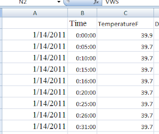
Figure 3. CSV File Exported to Excel

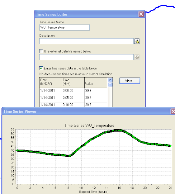
Figure 4:  Make a SWMM 5 Time Series to Copy and Paste the Temperature from the CSV File.

The data imported from the csv file to Excel and after the text to columns tool is used looks like this in Excel. The data is now ready to be imported into SWMM 5 as is by copying and pasting from Excel to a SWMM 5 time series file.  You need to perform the following steps:

1.     Make a new SWMM 5 Time Series,

2.     Copy and Paste the Temperature data from Excel to the SWMM 5 Time Series,

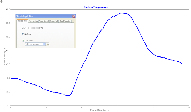
3.     Use the Climatelogy Data Tab and select the new Temperature Time Series as the source of the simulation temperature,

4.     You can see the simulated temperature by graphing the System Temperature.

Figure 5. SWMM 5 Climatology Tab and the resultant System Variable Graph of the Temperature.